The earliest application of the fundamental concepts of fluidization dates back to 16th century when a German scientist (Georgius Agricola) described a process to upgrade ores. However, it was not until the 1930s, with the development of the Winkler coal-gasification process, that commercial use of fluidized beds on an industrial scale was recognized. The need for gasoline during the World War II accelerated the development and implementation of the fluid catalytic cracking (FCC) process by a consortium of U.S. petrochemical and engineering companies.
During the past five decades, fluidization technology has been extensively applied to various chemical processes. It provides better heat and mass transfer between the fluid and the solid compared to conventional packed- or moving-bed unit operations. Some common industrial processes using fluidization technology include drying, catalytic cracking, chemical synthesis, adsorption-desorption, gasification, pyrolysis, granulation, calcination, combustion, coating, bioreaction, polymerization, ore beneficiation and coking. This article summarizes the basic concepts of fluidized-bed technology and provides a useful collection of equations for gas-solids systems.
Background
When particulate matter or bulk solids are poured into a vessel, the particles arrange themselves into a random configuration to form a fixed (or packed) bed. The space between the particles becomes filled with ambient gas and forms a network of interconnected voids. The volume occupied by the packed bed is always greater than the volume of the particulate material itself. The ratio of void volume to the total volume of packed bed is called voidage. Sometimes “porosity” is used to describe voidage of packed beds, but this should not be confused with porosity within the particles.
When a fluid (gas or liquid) is introduced uniformly at the bottom of the packed or fixed bed, it percolates upwards through the interstitial voids. The drag of the gas on the particles is counteracted by the pressure drop across the bed or the weight of the bed divided by cross-sectional area. The packing configuration of the bed remains unaltered as the fluid finds the tortuous path through the packing in the upward direction.
If the upward velocity of the fluid is increased such that the weight of the bed per unit cross-sectional area is equal to the pressure drop across the bed, then the particles begin to suspend and particle-particle contact is no longer assured. This condition is called minimum fluidization. Further increase in fluid velocity, will cause the suspended bed to exhibit “fluidity” or fluid-like behavior, creating the so-called fluidized bed.
Much like fluids, the particles in a fluidized bed can be stirred and discharged from a lateral orifice in the vessel. Particles of higher density will tend to sink while the lighter ones will tend to float to the surface of the bed. The top surface of a fluidized bed will be relatively horizontal (with an angle of repose of zero) and the particles will flow from a higher elevation to a lower elevation. Bubbling beds also have similar behavior as sparged liquid columns.
The behavior of the bed after minimum fluidization depends on whether the fluid is a liquid or a gas. For liquids, as the upward flow of liquid is increased, the packed bed continues to expand uniformly and homogenously with increasing interstitial void space until the particles are eventually carried away (elutriated) [ 9]. This type of fluidization behavior is called particulate or homogenous fluidization.
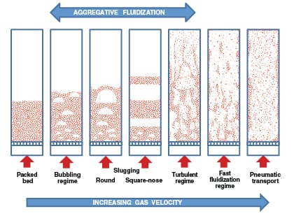
However, when the fluid is a gas, the excess gas may manifest itself as bubbles. The bubbles will result in two distinct phases within the bed and give an appearance of non-homogeneity. Such a behavior is called aggregative fluidization (Figure 1). Transition from a packed bed to either particulate or aggregative fluidization for gas-solid systems depends on particle and gas properties. To develop fluidized-bed processes for gas-solid systems, the ability to predict flow behavior and calculate essential operating parameters (such as minimum fluidization velocity, flow regimes, bubbling characteristics and more) is critical.
 |
|
FIGURE 1. Different fluidization regimes in gas-solid systems are demonstrated here (Image adapted
from [5] and [7] |
As shown in Figure 1, as the gas flowrate is increased in a bubbling gas-solid fluidized bed, the bubbles coalesce and may grow larger as they migrate to the bed surface (with coarse or granular solids) or achieve a stable size (with fine powders). The passage of bubbles through the bed will result in mixing and churning of the bed material, which creates uniform conditions within the bed. If the bubbles get larger than two-thirds of the bed diameter, slugging may result. Slugging conditions can cause severe pressure fluctuations and bed vibrations along with significant reduction in heat and mass transfer. Commercially scaled units for fine powders tend not to exhibit slugging. However, slugging behavior may be observed with coarse materials.
Further increase in gas flowrate and the onset of a turbulent regime is marked by the disappearance of a distinct bed surface. At this point, the void spaces and the particles form co-continuous phases. At higher velocities, the contents of the bed are elutriated (carried out of the vessel), thereby resulting in partial depletion of the bed material. This fluidization regime — also known as fast fluidization — is characterized by an axial concentration gradient, a subtle core-annulus profile and recirculation at the walls.
At even higher gas velocities, complete removal of the bed material can occur. The “bed” becomes divided between a developing flow and fully developed axial flow with a distinct core-annulus radial profile. This flow regime is referred to as the transport flow regime.
Geldart classification
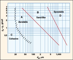
In 1973, Professor Derek Geldart proposed a simple and elegant approach for predicting the fluidization behavior of particulate materials in a classic paper [2]. He plotted the density difference between the solid phase and the fluid phase versus particle size on a log-log plot, and proposed four major classes (A, B, C and D) based on their fluidization behavior (Figure 2). These have come to be known as Geldart particle classifications.
 |
|
FIGURE 2. Geldart classification for fluidization characteristics in air at
ambient conditions [3] |
Since the density of gas is typically three orders of magnitude smaller than the density of particles, the particle density dominates the y -axis. The particle diameter on the x -axis refers to the surface-volume diameter ( d sv) for uniform-sized particles and the surface-volume mean diameter ( d svm) when the particles are non-uniform in size.
Typical characteristics of each of the Geldart classes are summarized here:
Class A
• Fine powders
• Easy to fluidize; aeratable
• Exhibit homogenous or particulate fluidization until bubbling
• The bubbling velocity is greater than the minimum fluidization velocity
• Good mixing occurs during complete fluidization
• Slow deaeration rate or long de-fluidization time observed
• Examples include fluidized catalytic cracking catalysts, high-density polyethylene powders and TiO2
Class B
• Granular appearance, sand-like
• Exhibit aggregative or bubbling fluidization from the onset
• Starts bubbling immediately after incipient fluidization
• Fast deaeration observed
• Examples include coarse sand, polymer granules, detergents, coal feeds and coke
Class C
• Fine ( d p<20 μm) and cohesive powders with high interparticle interaction
• Powders tend to channel during fluidization
• The bed may retain gas for extended periods (that is, may experience a long de-fluidization time)
• Usually requires flow aids for fluidization (such as vibration or additives)
• Examples include fine coal, carbon black, talc, flour, fumed silica and nanoparticles
Class D
• Large particles
• Solids tend to fluidize poorly or exhibit spouting
• Exhibits fast deaeration
• Examples include plastic pellets, rocks, pebbles, grains and seeds
 |
|
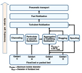
FIGURE 3. Shown here are the typical transitions between various fluidization regimes
|
 |
|
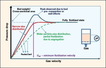
FIGURE 4. Shown here is a characteristic pressure drop response as the packed bed transforms to a
fluidized state with increasing gas velocity |
Not all of the fluidization regimes shown in Figure 1 are observed in practice. This depends on the Geldart classification of the material and the bed geometry (in terms of diameter and the height/diameter ratio). The typical flow regime transitions have been summarized in Figure 3.
Minimum fluidization velocity
Minimum fluidization velocity is the transition velocity at which packed-bed behavior changes to fluidized-bed behavior. It corresponds to the condition where the weight of the bed per unit cross-sectional area is equal to the pressure drop across it. The pressure drop increases linearly with gas velocity in a packed bed until the total drag force on the bed starts to approach the weight of the bed (Figure 4).
In beds with small bed diameter (<6 in.), the effective bed weight is slightly less than the calculated bed weight because the bed is partly supported by retaining walls due to friction, and by the distributor plate. If the bed is pre-compacted or the diameter is small, the pressure drop exhibits a peak value before settling into a largely constant value. For beds with wide particle-size distribution, the pressure drop curve will be broader without a distinct point of inflection.
The minimum fluidization velocity is estimated by linearly extrapolating the packed-bed characteristics and fluidization characteristics, and locating the point of intersection. This is shown in Figure 4 for an example with a narrow particle-size distribution.
The experiment to determine minimum fluidization velocity is best performed by first achieving a fully fluidized state, and then progressively decreasing the gas flowrate.
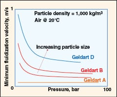
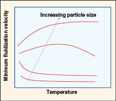
Pressure, temperature effects
High temperature and pressure conditions are common in commercial processes that use fluidized-bed technology. However, it is often difficult to conduct laboratory experiments at such elevated conditions. Knowlton (Chapter 2 in Yang [12]) provides an excellent review of the effect of temperature and pressure on the minimum fluidization velocity. Higher pressure increases the gas density with little change in viscosity, whereas higher temperature increases the viscosity but decreases the density. As a result, the combined effect of temperature and pressure changes often creates confounding effects on the actual state of fluidization.
 |
|
FIGURE 5. The effect of pressure on minimum fluidization
velocity is shown here (adapted from Yang [12]) |
 |
|
FIGURE 6. Shown here is the effect of temperature on
minimum fluidization velocity (adapted from Yang [12]) |
• Effect of pressure (as shown in Figure 5):
– The minimum fluidization velocity (Umf) is insensitive to pressure for fine powders (Geldart class A materials)
– Geldart class B and class D materials exhibit a decrease in Umf with pressure
• Effect of temperature (as shown in Figure 6):
– Umf decreases with increasing temperature for fine powders
– At intermediate particle size, the Umf exhibits a maximum value where viscous forces dominate at higher temperatures
– For larger particles, Umf increases with temperature due to a decrease in density
Particle characterization
Particle size.Size, shape, density and surface characteristics are key intrinsic parameters that dictate the response of a particle in a flow field. While one may use any average dimension of the particle to qualitatively reflect its size, a more precise and meaningful definition is required for calculation purposes.
The size of a spherical particle is uniquely determined by its diameter. Similarly, the size of regular isotropic particles (cylinders, cubes, spheroids) can be uniquely defined by two dimensions. In the real world, however, we deal with irregular three-dimensional particles whose “size” parameter must be uniquely determined. The most logical approach is to define an equivalent diameter that corresponds to a sphere and exhibits the same behavior as the irregular particle when subjected to a given physical process under consideration.
The most common equivalent diameters are briefly defined here. There are no definitive guidelines for the selection of the most appropriate diameter that applies for every situation.
Volume diameter (dv). The diameter of a sphere having the same volume as the particle is defined by Equation (1):
![]() (1)
(1)
Surface diameter (ds). The diameter of a sphere having the same surface area as the particle is defined by Equation (2):
![]() (2)
(2)
Surface-volume diameter (dsv). The diameter of a sphere having the same ratio of volume to external surface area as the particle. This is also known at the Sauter diameter, and is defined by Equation (3):
![]() (3)
(3)
A sphere is often used as the reference shape because of its theoretical and experimental convenience. Sieve diameter, Stokes’ diameter, Feret diameter, Martin diameter, Perimeter diameter, Chord and Projected area diameter are other notable equivalent diameters that are defined and used in the literature.
Mean or average diameter. Granular materials or bulk solids are an assemblage of particles of varying sizes and shapes. If we were dealing with a collection of uniform sized spheres, the mean or average particle size would simply be a function of the diameter of the sphere. If the bulk solid consists of spheres of varying sizes, then the appropriate average equivalent diameter must be calculated. Similarly, for bulk solids consisting of irregular particles one must first define a property of interest (volume, surface area), estimate the average value for the mixture and then calculate the diameter of the equivalent sphere with the same property value.
The surface-volume mean diameter [d svm; also called Sauter mean diameter, and defined in Equation (4)] is widely accepted and used as the equivalent average (mean) particle diameter for many fluidized bed applications, fluid-particle systems, bins, hoppers and chutes. It is mathematically equivalent to the harmonic mean diameter and can be approximated by the following equation:
![]() (4)
(4)
This definition can be applied to data gathered using sieve analysis or the laser-diffraction method.
A bed of spheres of dsvm equivalent diameter will have the same bed surface area per unit volume as the actual bed. This representation creates the necessary bias toward the finer fraction, which reflects the significance of fines in fluidized bed and bin and hopper operations.
A worked example. Calculate the surface-volume mean diameter (Sauter mean diameter) for a granular material using data from sieve analysis. The data and calculations are shown in Table 1.
| Table 1. Calculation of surface-volume mean diameter | ||||||
| Upper sieve size (Mesh) | Aperture size, micron | Lower sieve size (Mesh) | Aperture size, micron | Average particle size (dpi) | Weight fraction (xi) | xi / dpi |
| 20 | 833 | 28 | 589 | 711.0 | 0.10 | 0.00014 |
| 28 | 589 | 35 | 417 | 503.0 | 0.15 | 0.00030 |
| 35 | 417 | 48 | 295 | 356.0 | 0.27 | 0.00076 |
| 48 | 295 | 65 | 208 | 251.5 | 0.13 | 0.00052 |
| 65 | 208 | 100 | 147 | 177.5 | 0.10 | 0.00056 |
| 100 | 147 | 150 | 104 | 125.5 | 0.07 | 0.00056 |
| 150 | 104 | 200 | 74 | 89.0 | 0.09 | 0.00101 |
| 200 | 74 | 270 | 53 | 63.5 | 0.06 | 0.00094 |
| 270 | 53 | Pan | 0 | 26.5 | 0.03 | 0.00113 |
| Sum xi / dpi = | 0.00592 | |||||
| dsvm, micron = | 168.8 | |||||
Median diameter (d50). Particle diameter corresponding to 50% on the cumulative weight percent curve of particle size distribution. Similarly, d95 corresponds to 95% on the cumulative weight curve of particle size distribution.
Particle density. Particle density (ρp) is defined as the mass per unit volume of the particle. The space occupied by solid, open and closed pores is included in the volume calculation. This is the most commonly used definition of density in correlations. When the volume calculation only includes the volume of solid and closed pores, the corresponding density is called the skeletal density.
Particle shape.The shape factors are based on some combination of surface area, volume, projected area and projected perimeter. The relevance of a shape factor to an application depends on method of measurement and the critical attributes for process performance. For fluid-particle flow systems, namely packed beds and fluidized beds, sphericity (Ï•s) is most useful. It is defined via Equations (5) and (6):
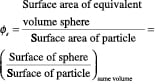 (5)
(5)
![]() (6)
(6)
The sphericity of a sphere is equal to 1. It is easy to calculate the sphericity of regular isometric particles (this is demonstrated in Table 2). It should be noted that various shapes can have the same sphericity value. Estimation of the sphericity of irregular particles requires measurement of the surface area of particles in the bed. In practice, effective sphericity is back-calculated from the system response (using, for example, the experimental pressure drop in a packed bed and Ergun’s equation [see Equation (24), below].
| Table 2. The sphericity of common particle shapes | ||
| Shape | Relative proportions | Sphericity (Ï•s) |
| Sphere | – | 1 |
| Spheroid | 1:1:2 | 0.93 |
| Spheroid | 1:2:2 | 0.92 |
| Spheroid | 1:1:4 | 0.78 |
| Spheroid | 1:4:4 | 0.7 |
| Ellipsoid | 1:2:4 | 0.79 |
| Cylinder | H = D | 0.87 |
| Cylinder | H = 2D | 0.83 |
| Cylinder | H = 4D | 0.73 |
| Cylinder | H = 0.5D | 0.83 |
| Cylinder | H = 0.25D | 0.69 |
Particle hydrodynamics
Terminal velocity and drag coefficient. When a single (isolated) particle is allowed to settle in a stationary infinite-fluid medium, it reaches a constant settling velocity where the gravitational force is balanced by the drag force and its buoyancy. This constant settling velocity is called the terminal velocity. The settling behavior of an ensemble of particles — the hindered settling behavior (discussed in greater detail below) — is affected by the concentration of the particles.
The forces acting on a particle moving relative to a fluid medium depend only on flow in the immediate vicinity. The drag coefficient for a single particle in an infinite medium is defined using Equation (7):
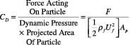 (7)
(7)
A simple definition of drag coefficient for Stokes regime (Re p<0.2) is found in Equation (8):
![]() (8)
(8)
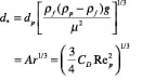
![]() (9)
(9)
 |
|
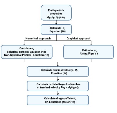
FIGURE 7. This generalized calculation scheme can be used to determine the terminal velocity and
drag coefficient |
 |
|
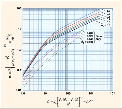
FIGURE 8. A dimensionless plot of characteristic velocity and particle size for isometric irregular
particles and disk-shaped particles is provided (Adapted from [7]) |
While Equation (9) is commonly used for quick estimation of terminal velocity, it does not address the conditions at higher Reynolds number and non-spherical shapes that are often encountered in practice.
A generalized approach for spherical and non-spherical particles. A generalized approach to calculate terminal velocity and drag coefficient in fluid-particle systems was proposed by Haider and Levenspiel [6] (see Figure 7). Characteristic curves with dimensionless particle size (d *) and velocity (u *) as the x – and y -axes, respectively, are plotted in Figure 8.
x-axis:
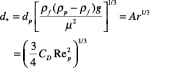 (10)
(10)
y-axis:
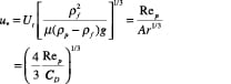 (11)
(11)
Where:
![]()
![]()
d p = Equivalent volume diameter (d v) of the particle.
The dimensionless velocity (u *) for spherical particle (Ï• s = 1) can also be calculated using Equation (12):
![]() (12)
(12)
For non-spherical isometric particle (0.5 < Ï• s ≤ 1), use Equation (13):
![]() (13)
(13)
Terminal velocity of the particle in an infinite medium can then be calculated using Equation (14):
![]() (14)
(14)
Richardson-Zaki Correlation for hindered settling. For multi-particle systems, the presence of neighboring particles affects the settling characteristics of all particles. The most widely accepted correlation for hindered settling was proposed by Richardson-Zaki [9]:
![]() (15)
(15)
The value of exponent n depends on the particle’s Reynolds number (Rep):
4.65 0 < Rep ≤ 0.2
4.35 Rep -0.03 0.2 < Rep ≤ 1
4.45 Re p -0.1 1 < Rep ≤ 500
2.39 Rep > 500
Drag coefficient (CD). Once terminal velocity is determined, the drag coefficient at the terminal velocity can be calculated using empirical correlations proposed by Haider and Levenspiel [6].
Spherical particles:
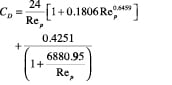 (16)
(16)
Non-spherical (isometric) particles:
 (17)
(17)
Where:
![]()
Worked example:
Data:
Particle size (volume equivalent diameter), dp = 1 mm = 0.001 m
Particle sphericity, Ï•s = 0.7
Particle density, ρp = 2,500 kg/m3
Fluid density, ρf = 1,000 kg/m3
Fluid viscosity, μ = 1.002 cP
= 1.002 x10⁻³ kg/(m.s) or (N s/m2)
Solution:
d * = 24.226
u * = 4 (graphical)
u * = 3.891 (equation)
U t = 0.096 m/s
Rep= 95.57
CD = 1.250
Packed-bed hydrodynamics
Packed-bed voidage. A packed bed of particles always has free space or voids between the particles. The relative amount of voids, which is called voidage (εb), depends on the nature of packing and can be determined using Equation (18). Regular hexagonal packing (εb = 0.26) and regular cubic (εb = 0.48) define the two bounds of voidage for mono-sized spherical particles.
![]() (18)
(18)
Bulk density, particle density and bed voidage are inter-related:
![]() (19)
(19)
![]() (20)
(20)
 |
|
FIGURE 9. The relationship between bed voidage and particle shape is shown here
|
Using Brown’s data [1] (d p > 500 μm), we have developed the following correlations for a randomly packed bed (Figure 9):
![]() (21)
(21)
![]() (22)
(22)
![]() (23)
(23)
When the bed diameter is greater than 30 times the particle diameter, the wall effects can effectively be neglected. It has also been observed that the local voidage at the wall (extending up to 6 particle diameters) will be lower than the bulk value. It is interesting to note that the packed-bed voidage is independent of particle size, as long as the interparticle forces are relatively insignificant, which is the case for most coarse, granular materials.
Pressure drop across the packed bed. There are two major approaches for modeling pressure drop across packed beds — using the channel-flow analogy model and using discrete-particle analysis. The channel-flow analogy models the flow similar to frictional flow in pipe channels where the tortuosity and variations in channel diameter are taken into consideration. The classic approaches of Carmen, Kozney and Blake are good examples of this approach (see Yang [13] for details).
Conversely, the discrete particle- analysis approach, which includes the analysis of the impact of drag forces and boundary layers on individual particles, is suitable for applications with higher Reynolds number and higher voidage values.
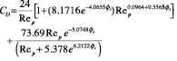
Ergun equation. The empirical approach proposed by Ergun in 1952 [3,7,13] has found widest acceptance, as it is based on a large amount of diverse data for Geldart Class A and B particles. He retained the basic dimensionless variables used in the channel-flow analogy but proposed empirical constants for the viscous and kinetic terms.
 (24)
(24)
The first term is the viscous term, and the second term is the kinetic term.
![]() (25)
(25)
![]() (26)
(26)
Use (+) for upflow and (–) for downflow configurations.
For a bed of spheres with uniform size, the particle size (dp) can be unambiguously specified as the diameter of the sphere. For a bed of non-spherical (isometric) particles of uniform size, the equivalent volume diameter (d sv=Ï• s. d v) should be used for dp. When the bed is composed of particles of different sizes and shapes, one must estimate a relevant equivalent-mean particle size (dsvm), which will result in the same specific pressure drop per unit volume as the given bed. The equivalent-mean diameter is given by Equation (27):
![]() (27)
(27)
Where x i is the weight fraction corresponding to particle size dpi. The calculation procedure is similar to the one outlined for dsvm earlier.
Since experimental measurement of bed voidage (εb) is fairly simple and accurate, it is always recommended that the measured value be used. It can also be calculated using Equations (21) to (23).
The sphericity of a sphere is 1. For irregular particles with an arbitrary shape, it is difficult to calculate sphericity from first principles. However, the effective sphericity of a bulk solid for packed-bed applications can be back-calculated from experimental measurement of pressure drop, which can then be used for subsequent predictions.
Worked example. Calculate the pressure drop across a bed of irregular particles:
Particle size, dv = 2 mm = 0.002 m
Particle sphericity, Ï•s = 0.8
Packed bed voidage, εb = 0.45
Bed height, H = 0.5 m
Fluid density, ρf = 1,000 kg/m3
Fluid viscosity, μ = 1.002 cP
= 1.002 x10⁻³ kg/(m.s) or (N s/m2)
Superficial velocity, Uf = 0.10 m/s
The calculations are summarized in Table 3.
| Table 3. Presssure drop calculations using Ergun’s equation | |||||
| Contribution, % | Pa or N/m2 | in. H2O | lb/in.2 | lb/ft2 | |
| Viscous effect | 20.4 | 9,744.89 | 39.16 | 1.41 | 203.63 |
| Kinetic energy effect | 69.3 | 33,007.54 | 132.65 | 4.79 | 689.74 |
| Static head | 10.3 | 4,905.00 | 19.71 | 0.71 | 102.50 |
| Upflow pressure drop = | 47,657.43 | 191.52 | 6.92 | 995.87 | |
| Downflow pressure drop = | 37,847.43 | 152.10 | 5.49 | 790.88 | |
Gibilaro equation. Gibilaro and others [4] proposed an improved equation to calculate pressure drop. It gives better predictions in both turbulent and laminar flow regimes for packed beds and expanded beds (εb> 0.5).
![]() (28)
(28)
Where:
![]()
The guidelines for choosing a representative particle size (dp) are the same as for Ergun’s equation.
Worked example. The worked example for Gibilaro’s equation uses the same data as shown for the example for Ergun’s equation, and the results are tabulated and shown in Table 4.
| Table 4. Presssure drop calculations using Gibilaro’s equation | |||||
| Contribution, % | Pa or N/m2 | in. H2O | lb/in.2 | lb/ft2 | |
| Viscous effect | 18.0 | 8,601.74 | 34.57 | 1.25 | 179.75 |
| Kinetic energy effect | 56.0 | 26,676.69 | 107.20 | 3.87 | 557.45 |
| Static head | 10.3 | 4,905.00 | 19.71 | 0.71 | 102.50 |
| Upflow pressure drop = | 40,183.43 | 161.48 | 5.83 | 839.69 | |
| Downflow pressure drop = | 30,373.43 | 122.06 | 4.41 | 634.70 | |
Fluidized-bed hydrodynamics
 |
|
FIGURE 10. Shown here is a flow regime map, according to Grace [5]
and Kunni-Levenspiel [7] |
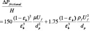
Flow regime identification. Extensive literature is available to provide guidance on how to identify the flow regimes for two-phase (gas-liquid) systems. For gas-solid flow, various flow-regime maps have been proposed using combinations of gas velocity, pressure drop, voidage, slip velocity, solids loading, Froude number and Reynolds number. The most comprehensive and practical flow-regime map was proposed by Grace [5] and later modified by Kunni-Levenspiel [7]. They plotted dimensionless superficial velocity ( u *) versus dimensionless particle diameter (d *) (Figure 10), and demarcated regions corresponding to the major flow regimes observed in gas-solid systems. This map applies to upflow conditions only. The approximate boundaries of Geldart’s classification can also be identified in the same plot. Once the x, y pair is located (Figure 10), the expected flow regime can be identified. Dimensionless particle diameter as x-axis:
 (29)
(29)
Dimensionless superficial gas velocity as y-axis:
![]() (30)
(30)
Worked example. Identify the flow regimes at various superficial gas velocities:
Data:
Particle density, ρp = 2,000 kg/m3
Gas density, ρf = 1.3 kg/m3
Gas viscosity, μ = 0.018 cP = 1.8 x10⁻⁵ kg/(m.s) or (N s/m2)
Particle size, dp (= d svm) = 80 μm
= 80 x 10-6 m
Acceleration due to gravity, g = 9.81 m/s2
Calculated d * = 3.426. Geldart classification: Type A. The results are summarized in Table 5.
| Table 5. Flow regime identification | |
| Gas velocity (Uf), m/s | Flow regime |
| 0.002 | Packed bed |
| 0.004 | Minimum fluidization |
| 0.15 | Bubbling bed |
| 0.80 | Turbulent bed |
| 1.70 | Fast fluidized bed/ Pneumatic transport |
| 5.0 | Pneumatic transport |
Minimum fluidization velocity.While the most reliable estimation of minimum fluidization velocity (Umf) is obtained experimentally (Figure 4), numerous researchers have proposed correlations for predicting it based upon fluid and particle properties [2, 7, 11, 12, 13 and 14].
We know that at the condition of minimum fluidization, the pressure drop across a bed is equal to the weight of the bed per unit cross-sectional area. Wen and Yu [11], using Ergun’s equation as the basis and making empirical substitutions for bed voidage and sphericity based on available data, proposed the following equation:
![]() (31)
(31)
Where:
![]()
![]()
For bulk materials with finite size distribution, it is recommended that readers use surface-volume mean diameter (d svm) as given by Equation (4) as the representative particle size dp.
Re-arranging Equation (31), minimum fluidization velocity can be calculated as follows:
![]() (32)
(32)
Subsequently, numerous researchers have correlated their respective data sets and come up with alternate constants (Table 6). A generalized version of Wen and Yu’s correlation can be written as follows:
| Table 6. Coefficients for generalized version of minimum fluidization correlation [7, 11,12] | ||
| Researcher | C1 | C2 |
| Wen and Yu | 33.7 | 0.0408 |
| Chitester et al. | 28.7 | 0.0494 |
| Grace | 27.2 | 0.0408 |
| Saxena and Vogel | 25.3 | 0.0571 |
| Babu et al. | 25.25 | 0.0651 |
| Richardson | 25.7 | 0.0365 |
| Thonglimp | 31.6 | 0.0425 |
| Bourgeois | 25.5 | 0.0382 |
| Lucas | 25.2 – 32.1 | 0.0357 – 0.0672 |
![]() (33)
(33)
![]() (34)
(34)
For Geldart A and B materials, Wen
and Yu’s correlation is recommended, while Chitester and others [7] is recommended for Geldart D materials.
Wen and Yu’s approach, while widely used and accepted, still remains controversial. It should be noted that they reported 34% standard deviation for their data set. Therefore, sufficient safety factors must be used when designing processes based on any of these correlations. Whenever feasible, it is recommended that minimum fluidization velocity be experimentally measured.
Worked example.
Data:
Particle density, ρ p = 2,000 kg/m3
Sphericity, Ï• s = 0.75
Gas density, ρf = 1.3 kg/m3
Gas viscosity, μ = 0.018 cP
= 1.8 x10⁻⁵kg/(m.s) or (N s/m2)
Particle size, d p = 200 μm =
200 x 10–6 m
Acceleration due to gravity, g = 9.81 m/s2
Solution:
Archimedes number, Ar = 629.37
Minimum fluidization velocity (per Wen and Yu) = 0.0262 m/s
Complete fluidization velocity. Complete fluidization velocity is calculated by substituting d svm (or Sauter mean diameter) by d 95 in the correlation for minimum fluidization. This velocity is often used to define the operating point of fluidized bed processes.
Comment on distributor design. To achieve uniform distribution of gas in a fluidized bed, it is recommended that the pressure drop across the distributor be at least 30% of the bed pressure drop, or at least 10 in. H2O column (2,500 Pa) on an absolute basis. More in-depth discussion on distributor design can be found in Yang [ 12].
![]()
![]()
Summary
Despite eight decades of research and development of powerful computer tools, the core of fluidization technology remains largely empirical. Scaleup and design of large-scale processes based on small-scale cold flow data still remains a challenging problem.
In this article, we have touched upon key concepts of fluidization technology and summarized key equations for particle characterization, particle and bed hydrodynamics. For in-depth understanding of the subject, the books by Geldart [3], Kunni-Levenspiel [7], Yang [11, 12] and Zenz-Othmer [ 14] are excellent resources. n
Acknowledgement
We appreciate the valuable comments and suggestions offered by Ray Cocco, president and CEO of Particulate Solid Research Inc. (Chicago, Ill.).
References
1. Brown, G.G. and others, “Unit Operations,” Wiley, New York, 1950, pp. 210–216.
2. Geldart, D., Powder Technology, Vol. 7, 1973, pp. 285–292.
3. Geldart, D. (ed.), “Gas Fluidization Technology,” John Wiley & Sons, 1986.
4. Gibilaro L.G. and others, Chem. Eng. Sci., Vol. 40, 1985, pp.1817–1823.
5. Grace, J., The Canadian Journal of Chem. Eng., Vol. 64, June 1986, pp. 353–363.
6. Haider, A. and Levenspiel, O., Powder Technology, Vol. 58, 1989, pp. 63–70.
7. Kunni, D. and Levenspiel, O., “Fluidization Engineering” (2nd Ed.), Butterworth-Heinemann Series in Chemical Engineering, 1991.
8. Pell, M., “Gas Fluidization,” Elsevier, 1990.
9. Richardson, J.F. and Zaki, W.N., Trans. Instn. Chem. Engrs., Vol. 32, 1954, pp. 35–53.
10. Turton, R. and Levenspiel, O., Powder Technology, Vol. 47, 1986, p. 83.
11. Wen, C.Y. and Yu, Y.H., AIChE Journal, May 1966, pp. 610–612.
12. Yang, W.C. (Ed.), “Fluidization, Solids Handling and Processing,” Noyes Publication, 1999.
13. Yang, W.-C. (Ed.), “Handbook of Fluidization and Fluid Particle Systems,” Marcel-Dekker Inc., 2003.
14. Zenz, F.A. and Othmer, D.F, “Fluidization and Fluid-Particle Systems,” Reinhold Chemical Engineering Series, 1960.
Authors

Shrikant V. Dhodapkar is a fellow in the Dow Elastomers Process R&D Group at The Dow Chemical Co. (Freeport, TX 77541; Phone: 979-238-7940; Email: [email protected]) and adjunct professor in chemical engineering at the University of Pittsburgh. He received his B. Tech. in chemical engineering from I.I.T-Delhi (India) and his M.S.Ch.E. and Ph.D. from the University of Pittsburgh. During the past 20 years, he has published numerous papers on particle technology and contributed chapters to several handbooks. He has extensive industrial experience in powder characterization, fluidization, pneumatic conveying, silo design, gas-solid separation, mixing, coating, computer modeling and the design of solids processing plants. He is a past chair of AIChE’s Particle Technology Forum.

Abdolreza (Abdi) Zaltash is senior researcher in the Building Equipment Research Group at Oak Ridge National Laboratory (Oak Ridge, TN 37831; Phone: 865-574-4571; Email: [email protected]). He received his Ph.D. in chemical engineering, M.S. in chemical and petroleum engineering, and B.S.Ch.E. from the University of Pittsburgh. His major research contributions are in the fields of heat activated technologies and CHP. He has served as a member of several ASHRAE technical committees (Cogeneration Systems and Absorption and Heat Operated Machines) and contributed in the re-write of Chapter 7 of t