Equilibrium stage simulations are the nearly universal process design tool for mass transfer columns that contact vapor and liquid in countercurrent flow. Whether the service is absorption, stripping, distillation, fractionation, quench or evaporation, equilibrium stage models make mass and heat balances easy. They quickly estimate stream conditions and physical properties. They are easily altered, so a change to any design parameter can be instantly assimilated into equipment and stream properties.
When it comes to the actual design of mass transfer columns, however, the use of theoretical stage simulations can leave engineers perplexed about what packing height to use, and can lead engineers to believe that packing efficiency is a bewildering art devoid of logic. A better procedure begins with process design by equilibrium stages, followed by conversion of theoretical stages to transfer units, followed by equipment choice and design. This procedure results in complete process design, correct expression of the mass transfer task and logical choice of equipment.
Limitations of equilibrium stages
Many packed column designs for distillation, absorption and stripping follow this path:
1. The task of the column is first defined by an equilibrium stage simulation. (Equilibrium stages are also called theoretical stages or theoretical plates.)
2. The column task is expressed as a profile of column internal loadings and as the theoretical stage needs of the column.
3. Packing rating software is used to choose a packing and a column diameter and to estimate the packing pressure drop.
Then comes the question: What HETP (height equivalent to a theoretical plate) will convert the equilibrium stage needs into packed bed depths? The answer to this question often seems unattainable and vague, and it may seem to lack engineering principle.
You may have heard statements such as, “The HETP of this packing in low-relative-volatility distillation is 300 mm.” What about other services, such as absorption, stripping, and high-relative-volatility distillation?
You may have heard that the HETP for a specific service is two or three times the HETP shown in published literature or in a standard packing test. Why is there such a difference? Is the proposed packing inferior? Is the recommended HETP excessively conservative? Are the published data grossly optimistic?
Some equipment design equations separate the magnitude of an assigned task from the performance of the equipment. In a simplified example of single-phase heat exchanger design, the required task can be described as a heat duty (Q) and the log mean temperature difference (LMTD); these issues have nothing to do with equipment. The exchanger performance is described as an overall heat transfer coefficient (U). Together, the required task and the exchanger performance indicate the required heat-transfer surface area (A):
A = (Q / LMTD) / U (1)
With similar rationale, many column designers think that the number of theoretical stages (NTS) is a complete description of the mass transfer task. They view HETP as a property of the packing. They believe that they have separated the task from the equipment performance by counting theoretical stages and then asking for the packing HETP to find the total packed bed height (H).
H = HETP X NTS (2)
But the number of theoretical stages does not completely define the task of the packing. The statement of required stages and the subsequent question of HETP have not properly separated equipment performance from the task to be done. So the HETP value needs to contain a correction for a poorly quantified task. HETP values can seem illogical because the HETP is not just a property of the packing; it also depends on the task to be done, and on how poorly NTS has quantified the task!
Mass transfer refresher
The mass transfer concepts and equations used herein are covered thoroughly in various mass transfer textbooks, including Treybal [ 1] and Henley and Seader [ 2]. These texts also describe the McCabe-Thiele [ 3] binary distillation diagram, which illustrates distillation stages and equilibrium driving forces. Figure 1 shows an example McCabe-Thiele diagram for a 20-stage distillation.
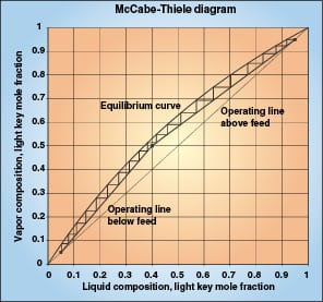
Above a column feed, we focus on purification of the vapor and on vapor composition (y). The vertical distance between the operating line and the equilibrium line represents the composition driving force for mass transfer, (y *– y). One equilibrium stage is movement of a distance (y *– y) along the operating line, where y and y * are measured at the beginning of the stage. The binary McCabe-Thiele diagram shows x and y values of the light component, but we are more interested in the values of y, y *, and (y – y *) for the heavy key component.
Below the feed, we focus on purification of the liquid and on liquid composition x. The horizontal distance between the operating line and the equilibrium line represents the composition driving force for mass transfer, (x – x *). One equilibrium stage is movement of a distance (x – x *) along the operating line, where x and x * are measured at the beginning of the stage.
Transfer units
In most packed columns, the mass transfer rate can be expressed by Equation (3) for the heavy key or absorbed component in the vapor, or Equation (4) for the light key or stripped component in the liquid. Elevation (h) is positive in the direction of flow, which is upward for vapor and downward for liquid.
Vapor mass transfer rate (G)
– G dy = KyaS (y – y *) dh (3)
Liquid mass transfer rate (L)
– L dx = KxaS (x – x *) dh (4)
The mass transfer coefficients K y and K x depend on many parameters, but not on x or y. In many columns, L and G are nearly constant over large sections of the column. (If this is not true, the adjustments do not change the major points of this paper, but they are not covered here.) Integration of Equations (3) and (4) provides the packed bed height H needed to change from composition Y 1 to Y 2, or X 1 to X 2:
For absorption and rectifying distillation columns:
![]() (5)
(5)
For stripping and stripping distillation columns:
![]() (6)
(6)
Number of transfer units (NTU).The above integrals in Equations (5) and (6) are dimensionless numbers called the number of transfer units, NTU OG and the NTU OL, respectively.
For the heavy key or absorbed component (NTU OG):
![]() (7)
(7)
For the light key or stripped component (NTU OL):
![]() (8)
(8)
Height of a transfer unit (HTU).The expressions outside the integrals of Equations (5) and (6) are called the height of a transfer unit, HTU OG and HTU OL, respectively. This paper focuses on columns where HTU can be estimated empirically, so we will not need terms like G, K y, L, K x, a and S.
H = HTU OG X NTU OG (9)
H = HTU OL X NTU OL (10)
The subscript O (for “overall”) indicates bulk phase compositions, not phase interface compositions. The subscripts G and L indicate use of y or x compositions, respectively.
Transfer units correctly separate the task (NTU) from the equipment performance (HTU). The task NTU depends on the compositions of the liquid and vapor, the relative volatility and the desired separation, but NTU has nothing to do with the equipment that must accomplish the task. The HTU depends on the packing, on flow rates, on physical properties and on liquid distribution quality, but it does not depend on the separation desired, the relative volatility, the reflux composition or the lean solvent loading.
Because transfer units are an accurate expression of a mass transfer task, HTU values will appear more sensible and more consistent than HETP values. This paper shows ways to evaluate the integral for NTU and provides guidelines to estimate the HTU values in various situations.
Low-Relative-Volatility Distillation
The McCabe-Thiele diagram in Figure 1 represents a hypothetical low-relative-volatility distillation column. It can also represent a packing efficiency test, although most efficiency tests occur at total reflux, where the operating line is the 45-degree line.
Consider one of the theoretical stages on the right side (above the feed) of the diagram. Note that the equilibrium line and the operating line are nearly parallel over the short range of each stage. This means that (y *– y) is constant at the beginning of the stage, in the middle of the stage, and at the end of the stage. Although the McCabe-Thiele diagram represents the light key compositions, it is also true for the heavy key component. The mass transfer driving force is the constant (y1–y2) over the entire stage.
Consider how many transfer units this theoretical stage represents. Because (y – y *) is the constant (y 1– y 2), Equation (7) reduces to:
![]() (11)
(11)
For low-relative-volatility distillation, each theoretical stage equals one transfer unit.So in low-relative-volatility rectification, the number of theoretical stages (NTS) is also the number of transfer units NTU OG. The equilibrium stage count NTS, which is important in mass and heat balances and in separation calculations, is the same as NTU OG, which is important to mass transfer. And, the HETP value is the same as the HTU OG value.
Over many years, hundreds of low-relative-volatility distillation tests have shown that many packings display about the same HETP over a wide range of systems and rates. Even widely varying pressure does not cause much HETP variation, although high pressures can imply high liquid rates that reduce the efficiency of structured packing. This principle has suggested the use of a single, characteristic HETP value for each packing. As an example, a structured packing product brochure [ 4] lists characteristic HETP values for two families of structured packing. This principle tends to apply to random packing and to sheet-type structured packing, but not to gauze and mesh type packing.
The consistency of HETP in low-relative-volatility distillation has simplified design of such columns, and engineers encounter few problems in proceeding from equilibrium stage calculations to packed bed heights. Engineers don’t even think about transfer units, and they don’t realize that the equivalence of equilibrium stages and transfer units has made their designs easier.
Low-relative-volatility distillation is not the focus of this paper. The topic of low-relative-volatility distillation is raised here because the hundreds of low-relative-volatility packing tests have provided a database of HTU OG values that are useful beyond the realm of low-relative-volatility distillation.
High-relative-volatility Distillation (Rectification Section)
Consider the rectifying section (above the feed) of a high-relative-volatility distillation column, and the heavy key component concentration in the vapor phase. Packing does not provide theoretical stages of vapor-liquid contacting. Packing simply contacts the two phases and lets the non-equilibrium compositions cause mass transfer between the phases. At any vapor-liquid interface in the column, the local mass-transfer rate is proportional to the driving force. In rectification, Equations (3), (5), (7), and (9) apply. We could reasonably say that packing provides transfer units, but not theoretical stages.
Counting theoretical stages does not take into account the effect of mass transfer progress on driving force. Theoretical stages set the mass transfer task of the packing in each stage according to the driving force of the incoming vapor. If the driving force diminishes as mass transfer proceeds in the packing, theoretical stages do not recognize the slowing of mass transfer in proportion to the diminishing driving force.
In the heat transfer analogy of Equation (1), suppose some illogical engineers decided to work with only one temperature differential (T – t)1 at one end of heat exchangers:
Q = U A (T – t)1 (12)
Suppose these engineers knew that (T – t) changes along the exchanger as heat transfer proceeds, but they refused to use an average (T – t), such as LMTD, instead of the fixed (T – t)1in Equation (12). Wouldn’t values of U vary severely to compensate for the error as (T – t)1 misrepresents the average (T – t)? Wouldn’t correlation and prediction of U be nearly impossible for heat exchanger design? This error and consequence are analogous to the error and consequence of using HETP in mass transfer.
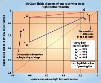 |
Figure 2 illustrates one equilibrium stage of a binary high-relative-volatility distillation. Vapor entering the stage has a driving force of 0.20, and 0.20 becomes the expected composition change of the stage. As mass transfer begins and the vapor moves up the operating line, the driving force declines. At the end of the stage, the driving force is only 0.04, so the mass transfer slows to one-fifth of the initial rate. Over the stage, the composition change of 0.20 must be attained with an average driving force much less than 0.20. This stage will require more packing than a stage in low-relative-volatility distillation, where the driving force stays constant over each stage.
Transfer units account for the change in mass transfer rate that is caused by changing driving force. We can evaluate the number of transfer units that the theoretical stage in Figure 2 represents for the heavy key component. Because the operating line and the equilibrium line are both locally straight, the integral in Equation (7) is simplified by the use of log mean driving force:
![]() (13)
(13)
Where
 (13A)
(13A)
The composition change (y 1– y 2) is (0.25–0.05) = 0.20. The log mean (y – y *) is the log mean of (0.25–0.05) and (0.05–0.01), or 0.0994. NTU OG is (0.20)/(0.0994) = 2.01. So the one theoretical stage in Figure 2 is two transfer units.
Evaluation of NTU OG for the rectification section of a distillation column is not difficult. An equilibrium stage simulation can provide the heavy key molar y compositions on each stage. The simulation is valuable in two respects:
1. It provides the y * equilibrium compositions above and below each stage; these are the y compositions on the next higher stages.
2. It divides the distillation into small pieces in which the operating and equilibrium lines are locally straight.
A spreadsheet can tabulate the heavy key y compositions stage-by-stage, the driving forces (y –y*) at the beginning and at the end of each stage, the log mean driving force over the stage, and the NTU OG for that stage. The sum of the NTU OG values of all the stages is the NTU OG of the column section.
Table 1 shows a simple rule that quickly converts theoretical stages to transfer units.
| Table 1. Quick Conversion Between Theoretical stages to Transfer Units | |
| If the key component declines by this factor from stage to stage: | Then the ratio of transfer units to stages, NTU/NTS, is: |
| 2.0 | 1.39 |
| 3.0 | 1.65 |
| 4.0 | 1.85 |
| 5.0 | 2.01 |
| 6.0 | 2.15 |
| 7.0 | 2.27 |
| 10.0 | 2.56 |
The database of low-relative-volatility packing tests can provide the HTU OG values for high-relative-volatility distillation. The characteristic low-relative-volatility HETP values are also more broadly applicable HTU OG values. Most high-relative-volatility distillation designs encounter flow conditions and physical properties that are well represented in the database, so the characteristic HETP is also the applicable HTU OG.
There are two ways to express the design of columns in high-relative-volatility systems.
1. Restate the theoretical staging needs as transfer units (NTU) and apply a consistent and repeatable packing HTU to the number of transfer units. This approach isolates the true difficulty of separation from the true performance of the packing. The packing performance as HTU can be adjusted for influences such as distribution quality, but the adjustments do not need to correct an understated task, so the HTU value will appear to be a reasonable number.
2. Continue to use theoretical stages (NTS) and apply a relative volatility correction factor to the packing HETP. In Example 1, this approach would state the separation task as three theoretical stages and the packing HETP as (2.01 multiplier) X (15 in. standard HETP) = 30 in. This traditional approach understates the separation difficulty as NTS, so the adjusted device performance HETP seems inconsistent with packing test data and with other uses of the packing. Without the above calculations, a 30-in. HETP in the example is certainly not obvious.
There are also two ways to determine the relative volatility effect:
1. Use the molar composition profiles of an equilibrium stage model to calculate the transfer units in each stage, as described above. Once understood, this is generally not a lengthy task. Another option is to use the multiplier in Table 1.
2. Use a mathematically equivalent approach to compute “lambda” λ = mG / L on each stage and use the following relation of NTS and NTU OG:
NTU OG = NTS (ln λ) / (λ–1) (14)
The correction can be applied to the HETP rather than the separation task:
HETP = HTU OG (ln λ) / (λ–1) (15)
In Example 1 and Figure 2, the value of m is 0.125 and L / G is 0.625, so λ is 0.20 and (ln λ)/(λ–1) is 2.01. Based on these values, the NTU is 6, the HETP is 30 in., and the bed depth is 90 in., just as previously calculated. Equilibrium stage simulations can be modified to calculate and tabulate values of λ and (ln λ) / (λ–1) automatically.
The effect of relative volatility on apparent packing efficiency as HETP is not new. The 1986 work of Koshy and Rukovena [ 5] applied λ correction factors to explain apparently poor packing HETP values in high-relative-volatility systems. The effect of relative volatility on packing HETP has become well known but is not well understood. Applying correction factors to the “packing performance” HETP does not clearly explain that equilibrium stages understate the separation difficulty, and the adjustment of apparent packing efficiency is trying to compensate for this understatement.
Absorption
Absorption processes are similar in some ways to rectification. But because the liquid phase is not limited to condensed vapor, there can be a wide range of liquid conditions. High liquid rate, high liquid viscosity, liquid-phase chemical reactions, limited solute solubility and extremes of “relative volatility” can affect mass transfer rates.
Few commercial absorbers contact vapor and liquid in near-equilibrium conditions. Most absorbers employ a solvent that exhibits little or no “back-pressure,” which is the equilibrium solute pressure over the partially loaded solvent; it indicates the tendency for absorbed solute to desorb back out of the solvent. So absorption can be similar to high-relative-volatility rectification in calculation of NTU.
Some absorbers employ solutions that have poor solubility for the solute, or they involve slow chemical reactions in the absorption process. Strigle [ 6] calls these columns “liquid-film-controlled” absorbers, and Equation (3) does not apply well. Sometimes the absorption rate is governed by a reaction rate rather than the mass transfer driver (y – y *). Maybe the equilibrium composition y * is zero in theory, after a reaction is complete, but is not zero at the point of mass transfer because the reaction is slow. Or the slow pace of solute acceptance in the liquid alters the mass transfer coefficients so that the HTU values are not predictable constants.
The classic example of a liquid-film-controlled absorption is the absorption of CO2 into weak caustic solution. The system is thought to be liquid-film-controlled because of the low solubility of CO2 in water. The CO2 molecules concentrate at the liquid surface, waiting for the solution to dissolve them as CO2 before converting them to carbonate. Once the CO2 is finally absorbed into the water, the caustic neutralizes it completely, thus giving the illusion of an excellent solvent with no back pressure.
This paper cannot address liquid-film-controlled absorbers, which evade broadly applicable design principles and require many individual approaches. However, most commercial absorption processes are not so complex. They involve simple mass transfer concepts wherein concentration driving forces cause mass transfer and the vapor-phase mass-transfer resistance controls the absorption rate. Designs do not involve reaction rate or liquid film control. As with high-relative-volatility distillation, theoretical stages understate the mass transfer task, but transfer units accurately express the task.
In many cases, an equilibrium stage simulation can establish mass and heat balances, compute the equilibrium relationship, and establish operating and equilibrium curves by dividing the overall absorption into smaller pieces. The NTU OG can be calculated for each stage, as described in the high-relative-volatility discussion.
The extreme theoretical stage dilemma occurs in systems with zero back pressure. The absorption of strong water-soluble acid vapors by caustic is an example. The acid reacts quickly and irreversibly with the caustic, and the still-alkaline solution has zero acid volatility. Because one theoretical stage is exactly 100% absorption, all such columns represent slightly less than one theoretical stage. This can create the illusion of a very easy absorption and a very short column. It can also create the illusion of high product purity, with 0.0 ppm of acid remaining in the vapor. For these reasons, an equilibrium stage simulation is ineffective for mass transfer design.
The extreme case of zero back pressure has a simple resolution. With no back pressure, y * is identically zero, and the definition of NTU OG in Equation (7) simplifies to:
![]() (16)
(16)
This is the common equation for “first-order decay.” Someone could have defined “HHL” as height of a solute half-life, or “H90” as height for 90% solute removal. (Actually there is an old rule-of-thumb that a 10-ft bed of packing provides 90% removal, two beds provide 99% removal, and so forth.) Nuclear first-order decay has taught that 100.000% removal (one theoretical stage) is never attained.
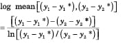
In some absorbers, the solvent load near the bottom of the column has significant back pressure, so transfer units in the bottom of the column must be calculated stage by stage using Equation (13). After the vapor passes through a zone of loading solvent, it passes into a zone where the solvent is lean and has little back pressure, so the remainder of the transfer units can be calculated from Equation (16).
The wide variety of absorber flow conditions can make the prediction of HTU OG complex. Some absorbers have flow conditions similar to those of the packing low-relative-volatility tests, so the expected HTU OG values will be like those of the test data. Other absorbers have conditions that differ from the distillation tests, so the test HTU OG values need adjustment. These adjustments can include the following:
• Upward adjustment for high liquid viscosity
• Upward adjustment for poor packing wetting with aqueous solvent
• Upward adjustment if the intended liquid distributor is imperfect
A high liquid rate in absorption service improves the HTU OG value by creating much surface area for the relatively slow vapor to contact, so distillation HTU OG values can be too conservative at high L / G.
Some companies or industries have packing efficiency data in various services. Measured HTU OG values are more applicable to other designs and columns than are HETP values. Because absorption HETP values contain corrections for poorly quantified mass transfer tasks, they are not useful in other columns unless they replicate the error too!
 |
|
Figure 3. A complex absorption can include a column zone of zero back |
Liquid and Vapor Film Resistances
Discussion of liquid stripping will require considering the individual film resistances of vapor and liquid, and their relative contribution to overall mass transfer.
Two-film theory of mass transfer divides the mass transfer process into two resistances: the liquid phase resistance and the vapor phase resistance. It says that the phase interface resistance is negligible, so that equilibrium is reached at the interface. There is a concentration gradient of x in the liquid phase, an equilibrium between x and y at the interface, and a concentration gradient of y in the vapor phase. The concentration gradients can be expressed in terms of resistance to mass transfer in each phase.
HTU values can be broken into individual phase components:
HTU OG = HTU G + λ HTU L (17)
HTU OL = HTU L + (1/λ) HTU G (18)
Note that in the extreme of low-relative-volatility distillation, λ = 1 and
HETP = HTU OG = HTU OL
= HTU G + HTU L (19)
In distillation, the value of HTU G is usually greater than HTU L. This implies that the liquid phase spreads thinly over the packing, it turns over quickly, and it builds little gradient between the interface and the bulk liquid. The vapor phase, however, does not quickly saturate the interface, so there is a larger concentration gradient between the bulk vapor and the interface, and more packed height is needed for mass transfer.
The low-relative-volatility distillation database says more about HTU G values than HTU L values. The observation about consistent low-relative-volatility HETP values over various rates and systems must apply to HTU G values too, because HTU G is the largest component of HETP. But the consistency of low-relative-volatility HETP values does not necessarily apply to HTU L values. HTU L values could vary within the database with little effect on HETP values, because HTU L contributes little to HETP.
High-relative-volatility Distillation — Stripping Section
The above high-relative-volatility distillation discussion focused on the rectification section only. The stripping section involves similar concepts and equations, but uncertainty over HTU L values makes calculations more uncertain.
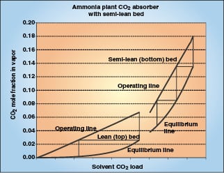
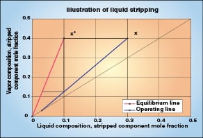
Figure 4 illustrates one theoretical stage of the stripping section of a high-relative-volatility distillation. The driving force (x – x *) is the horizontal distance between the equilibrium and operating lines. As in the rectification case, the driving force is large at the beginning of the stage, but it declines as mass transfer occurs and the liquid moves down the operating line.
As with y values in rectification, the number of transfer units (NTU OL) can be evaluated with x compositions of the light key component as it is stripped from the liquid. Possible techniques include using an equilibrium stage simulation and a spreadsheet as described above, or using Table 1 again, or evaluating λ on each stage and applying the λ correction factor in Equation (20).
NTU OL = NTS λ (ln λ) / (λ–1) (20)
For high-relative-volatility rectification, direct application of HETP values from low-relative-volatility test data as high-relative-volatility HTU OG values was really a minor conservative approximation. A more exact approach is to use HTU G and HTU L values to recalculate HTU OG in Equation (17). The value of HTU OG will decline slightly, as λ could decrease from near unity in low-relative-volatility rectification, to a value well below one for high-relative-volatility rectification. Because the individual HTU G and HTU L values are unknown, the exact amount that HTU OG will decline is unknown. But the decline will be small because HTU G is larger than HTU L.
The stripping section of high-relative-volatility distillation can similarly use the HTU G and HTU L values from low-relative-volatility distillation in Equation (18). In high-relative-volatility stripping, the λ value may increase from near unity to a value well above one. This decreases the value of HTU OL by decreasing the second term in Equation (18). Because the larger of the two terms is the one that declines, the magnitude of the decline of HTU OL is unknown; it may or may not be small. Using the HETP value from the low-relative-volatility distillation data as an approximate HTU OL value in high-relative-volatility stripping could be conservative. Koshy and Rukovena [ 4] illustrated this effect when they found that minimum HETP values do not occur at λ = 1, but at λ > 1.
In the above situation, an engineer could choose to use the low-relative-volatility HETP as a conservative HTU OL value, to avoid a difficult search for sources of HTU L or HTU OL data or Kxa data.
Reboiled Liquid Stripping
In reboiled strippers, the liquid mixture is at its boiling point and the vapor is composed of the same components as the liquid. In most reboiled strippers, the flow conditions, physical properties, and equilibrium conditions are similar to those of the stripping section of a high-relative-volatility distillation column. Reboiled strippers can generally be addressed by the techniques and calculations of the “High-relative-volatility distillation — stripping section” discussion above.
Liquid Stripping with Steam or Inert Gas
As the above discussion moved from high-relative-volatility rectification to absorption, counting transfer units NTU OG stayed the same, but the variety of potential solvents presented challenges in finding HTU OG values. Similarly, for liquid stripping that is not reboiled in stripping of bubble point liquid, counting transfer units NTU OL stays the same, but there are problems finding the HTU OL value for the stripper.
In strippers that use steam or other light gas to strip light compounds from a liquid mixture, the liquid mixture is not at bubble point, so its viscosity can be high. Many such strippers operate with little stripping gas and with little solute stripped, so that L / G ratios can be very high, vapor rates can be very low, and liquid rates can be very high. The distillation data that suggested HTU values in other columns are not helpful in suggesting HTU OL values under these conditions.
This article does not have approximations of HTU OL for the wide variety of strippers represented in this category of mass transfer. However, high volatility and few stages are not indicators of a trivial task, and an accurate NTU OL count and a reasonable HTU OL approximation are needed. A 2007 paper by Lopez-Toledo [ 7] and others at The Dow Chemical Co. presents a general correlation for k L values that can be used to build HTU OL for stripping service.
If a stripping column is large and a conservative approximation is too expensive, the situation could justify research and testing to measure HTU OL values. This situation occurred several years ago when an entire industry needed design data for stripping VOC (volatile organic compounds) from contaminated groundwater. The magnitude of the need justified many packing tests.
Distillation Trays
This article has not addressed trays, as opposed to packing, as the mass transfer device. However, nothing in the analysis of driving forces and nothing in the counting of transfer units is specific to the type of mass transfer device. As with packing, equilibrium stages are a poor representation of the mass transfer task of trays, and tray efficiencies must account for this. For that reason, trays with good bubbling activity and tall weirs can exhibit tray efficiencies of 25% in absorption service. The 1946 O’Connell [ 8] tray efficiency correlation has a relative volatility effect, because high relative volatility implies low “apparently poor” tray efficiency.
There may be a perception difference between packing and trays, in that 25% tray efficiency in absorption service is not perceived to indicate poor performance of the tray, but a packing HETP of 2,000 mm is often perceived as poor performance. Designers may accept without question the premise that 12 trays are needed for one or two absorption stages, or 20 trays for three absorption stages. An understanding of transfer units will help explain tray efficiency under high-relative-volatility and absorption conditions.
References
1. Treybal, Robert, “Mass-Transfer Operations,” McGraw-Hill, Third Edition, 1980.
2. Seader, J.D. and Henley, Ernest J., “Separation Process Principles,” John Wiley & Sons, 1998.
3. McCabe, W. L. and E. W. Thiele, “Industrial Engineering Chemistry,” 17, 605 (1925).
4. “INTALOX® Packed Tower Systems – Structured Packing,” Koch-Glitsch Brochure KGSP-1, page 5.
5. Koshy, T. D. and Rukovena, Frank, Reflux and Surface Tension Effects on Distillation, Hydrocarbon Process., May 1986.
6. Strigle, Ralph F., “Packed Tower Design and Applications,” Gulf Publishing, Second Ed., 1994.
7. Lopez-Toledo, Sawant, Castillo, Au-Yeung, and Pendergast, A.I.Ch.E. Annual Meeting, Salt Lake City, UT, November 2007.
8. O’Connell, H. E., Trans. A.I.Ch.E., 42, 741 (1946).
Author
Kenneth Graf is a principal engineer at Koch-Glitsch, LP (4111 East 37th Street North, Wichita, KS 67220; Email: [email protected]). Ken graduated from the University of Akron (Akron, Ohio) with a B.S.Ch.E. degree is 1977 and an M.S. degree in 1984. Since 1977, he has worked with distillation equipment (column trays and packing) at the Standard Oil Co. (Sohio), Norton Co., Saint-Gobain NorPro, and Koch-Glitsch, LP. Graf has designed many columns for the petroleum refining, ethylene and chemical industries.