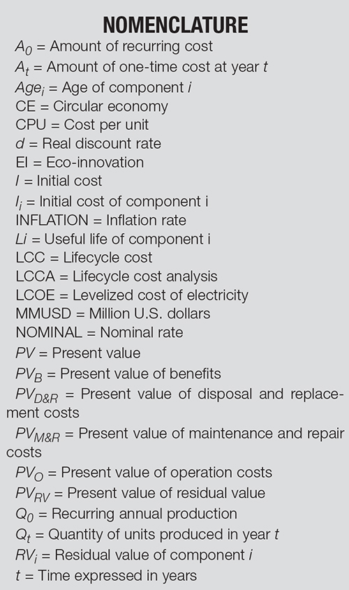
Lifecycle cost analysis (LCCA) can be used as a tool for selecting alternatives that add the most value to a project. The methodology for implementing LCCA is described here
In the chemical process industries (CPI), identifying optimum process designs challenges both process and cost engineers: the first must optimize the process in terms of throughput rate, process yield and product purity (among other factors), whereas the second are responsible for estimating the costs of the different design alternatives to allow assessing their impact against the business case. Their close interaction from the beginning of the project is key, as the ability to impact cost and functional capabilities is highest in the project’s early stages, where the cost of design changes is lowest [1].
The types of choices the design team takes throughout project development usually include: location, capacity, technology and process configuration (typically at the visualization/conceptual phase), equipment types and specifications, layout definition, utilities (typically at the conceptual/ basic engineering phase), vendor selection, construction methods, logistics and general planning (typically at the detail engineering/procurement/construction phase), and operational improvements (during operation of the plant).
In some situations, the decision is taken based on the lowest price (or lowest initial cost). This approach is better suited when comparing different bidders offering the same product or service, with little differentiation amongst the bidders (for example, civil works, where the design drawings and quantities of materials have been previously defined and included in the scope of the contract, and the bidders are selected from a short list of pre-qualified firms).
In other scenarios, there may be important differences between the evaluated alternatives in terms of capital, operations and maintenance and decommissioning costs. Here, being “cost effective” no longer means considering only the initial cost of an investment, but rather the investment throughout its entire useful life. In these cases, other techniques are better suited, such as: evaluation matrix, value-improvement practices, cash flow analysis or lifecycle cost analysis (LCCA).
The present article focuses on LCCA as a tool for selecting alternatives that add the most value to a project, describing a basic methodology for implementing an LCCA, with some examples of applications in the CPI.
LCCA basics
 To put it simply, the purpose of a LCCA is to enable the project design team to select the alternative with the “least long-run cost” [2] and obtain the same end goal. This is done by comparing the different alternatives on a common base: total levelized cost, which adds initial and future project costs, adjusted to take into consideration the time value of money.
The LCCA can be applied to several if not all parts of the project. As the main goal of this analysis is to provide several alternatives to pick from, the main challenge for the project design team is to find the effects of these options [3].
For example, when planning for a building, the LCCA is used to analyze the best options for transportation, materials and workforce, and it also takes into consideration the future maintenance and operational costs of the same building along with the disposal of materials that might have once been in the area (debris, trees and so on). Similarly, this method can be applied to chemical process facilities to analyze either the entire process, sections of the process, or its unit operations (for example, reactors, heaters, pumps) individually.
There are several factors that are taken into consideration when developing an LCCA, but the basics of this analysis lay on quantifying the present value of initial, operation, maintenance and repair, disposal and replacement costs, residual value and any benefits associated with each alternative, adding them along the life of the project and comparing them to the base case. To simplify the analysis, the team performing the LCCA may consider only the differences in each cost category between each evaluated alternative.
As the LCCA takes into consideration several components of a project, it is important to keep in mind that costs “are considered to be significant when they are large enough to make a big difference in the lifecycle cost” (LCC) [3], that all costs are expressed in the unit base-date currency (for example, December 2020 dollars) and that the analysis should consider the longest running part of the project (that is, if the study period is set for a time span that is shorter than the plant useful life, then the remaining useful life can be included in the analysis by means of the residual value).
Hence, even though there are different ways to determine the LCC of a project, a general formula for the LCC can be that shown by Equation 1:
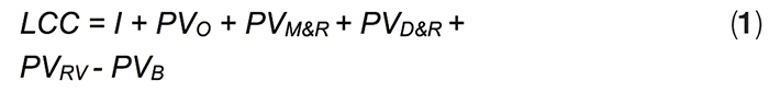
Where:
LCC = Lifecycle cost
I = Initial cost
PVO = Present value of operation costs
PVM&R = Present value of maintenance and repair costs
PVD&R = Present value of disposal and replacement costs
PVRV = Present value of residual value
PVB = Present value of benefits
The components of Equation (1) are described below:
Initial cost. The initial cost includes all capital investments to be made until the project is operational. This includes direct costs, such as equipment, materials, buildings and construction work, as well as indirect costs, such as lease, studies, permits, engineering, project management, taxes and overhead. To estimate this cost, cost engineers will require data regarding the scope and characteristics of the facilities to be constructed (such as equipment list, materials lists, work quantities) along with construction cost data with sufficient detail according to the project phase and desired precision.
Operation cost. Operation costs include all the annual costs required to run the facility, excluding maintenance and repair costs. These include raw materials, utilities (water, electricity, gas and so on), operational labor and services, and indirect costs (such as lease, insurance, security, royalties, overhead). To estimate these costs, process engineers need to develop estimates of the consumption of raw materials, chemicals and catalysts (as applicable), consumables, utilities, and workforce, whereas cost engineers need to gather data on their suppliers, local rates, as well as that of indirect costs.
Maintenance and repair cost. Maintenance and repair costs deal with the upkeep of the project itself and take into consideration that some of these costs can be annual or scheduled at several-year intervals into the future. Mechanical, instrumentation and electrical engineers may provide information regarding the maintenance requirements and frequency of the equipment involved in the project, while civil engineers may provide information about maintenance requirements for building, foundation and structural components; cost engineers then need to estimate rates and work hours for the required maintenance tasks.
There is also a risk factor to account for non-scheduled repairs (that is, corrective maintenance and resulting loss of production) that depends on failure rates of pieces of equipment. In a more detailed LCCA, this information may take into consideration results from a reliability, availability and maintainability (RAM) study.
Downtime costs (for example, loss of production, penalties and so on) due to maintenance and repairs may also be considered, if found to be significantly different between the evaluated alternatives. Process engineers usually estimate the quantity of production lost by downtime, whereas cost engineers evaluate their prices, and any penalties that may result.
Disposal and replacement costs. Disposal costs deal with the removal of existing structures or nature on site along with the transportation of wastes generated by construction or demolition (debris, residues and so on). More importantly, however, are the replacement costs. Every component of a project has a useful life, and the replacement costs are generated by removing and replacing components of the project that have completed their useful lives [4]. To estimate these costs, cost engineers will need, along with the list of equipment, materials and work to be installed (provided by the design team to estimate the initial costs), the useful life of each component.
Residual value. The residual value includes costs associated with the project after the study period is over. These values may be positive, negative, or zero. If the values are positive, it means that there are disposal costs attached to the end of the project (for instance, remediation costs), whereas negative values mean there is value linked to the facility at the end of the study period (for example, the plant has a useful life that exceeds the study period) and a zero value indicates no value associated at the end of the study [5].
For any component of the project whose useful life exceeds the study period, its residual value may be estimated (assuming linear depreciation) by using Equation (2):
![]()
Where:
RVi = Residual value of component i
Ii = Initial cost of component i
Agei = Age of component i
Li = Useful life of component i
It is important to note that the residual value estimated by assuming linear depreciation may be considerably different from the market value that the asset will have at the end of the study period, so care should be taken when assigning this value.
Benefits. Benefits include any other value gained by the project throughout the project life. Only benefits that can be traduced into monetary value are included in the LCCA. For instance, the value of emission reduction certificates or tax incentives received from implementing one design alternative are taken into consideration. Improved image can be considered as a benefit, so long as it can be justified that it will result in improved sales or improved company value, but this is harder to demonstrate when performing projections. If the company is considering other benefits within its project evaluation criteria that cannot be directly converted to a monetary value, then the LCCA is typically accompanied by a weighed qualitative evaluation matrix to aid in the selection of the preferred design alternative.
Discount rate and present value
Present value is defined as the time-equivalent value of all cashflows from the start of the project [5]. As the general cost of the project is affected by costs incurred at project start (or the base year), and future costs (any year after the start of the project) these expenses have to be levelized.
Future costs are any costs incurred at any time between year one and the study period. They include recurring and one-time costs, affected by the discount rate.
One-time costs (for instance, replacement of a major equipment component) can be brought to present value using Equation (3). Recurring costs (for example, yearly operational costs) can be brought to present value using Equation (4).
![]()
Where:
PV = Present value
At = Amount of one-time cost at year “t”
d = Real discount rate
t = Time expressed in years
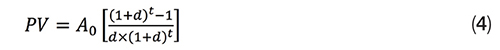
Where:
PV = Present value
A0 = Amount of recurring cost
d = Real discount rate
t = Time expressed in years
The effect of inflation on the real discount rate can be taken into consideration by using Equation (5).
![]()
Where:
d = Real discount rate
NOMINAL = Nominal rate
INFLATION = Inflation rate
Ref. 5 contains a more detailed discussion of time-value of money.
Levelized cost per unit
Another useful way to express LCC comes in the form of a levelized cost per unit (CPU). This is obtained by dividing the total lifecycle cost by the levelized units produced by the plant throughout the period in the study, yielding a value in terms of cost per ton, cost per barrel, cost per kilowatt-hour, or any other unit of significance to the plant output, as calculated on Equation (6). In Equation (6), it is worthy to note that production in future years is also adjusted using the discount rate.
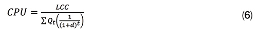
Where:
CPU = Cost per unit
Qt = Quantity of units produced in year t
If the annual production is assumed constant throughout the entire evaluation period, then Equation (6) can be simplified to Equation (7):
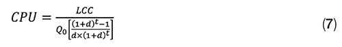
Where:
Q0 = Recurring annual production
The benefit of expressing the LCC in cost per unit form is that it allows the project design team to compare each option against benchmarks for other plants or technologies.
LCCA at different project phases
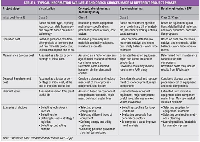
An LCCA may be performed at different project phases (for example, visualization, conceptual engineering and so on), with varying degrees of available information, to aid in different design choices. Table 1 shows an example of the type of information available and some typical choices that can be made with LCCA at different project phases (Note: this table is to be used as a general guideline only, as different information may be made available at different project stages depending on how the project is planned).
Examples of LCCA
The following examples of LCCA can be used to illustrate the usefulness of LCCA for some project design choices. The values in the following examples have been slightly altered or simplified from real project data for illustrative purposes.
Examples of LCCA 1: Reducing costs at an operating plant — energy recovery with a high-pressure gas expander. In this example, a high-pressure gas stream is currently being expanded in a pressure-reduction valve. Plant management is evaluating the installation of an expander to recover energy from the gas and use it to generate electricity that would be consumed inside the plant. The current electricity price forecast can be approximated as an average of $72/MWh (or 7.2¢/kWh) for the entire study period.
Based on the gas flowrate and process conditions, it is estimated that a 280-kW expander can be installed, with said expander being capable of generating 2,350 MWh of energy each year. The total cost of the installation, including procurement of equipment and materials, transportation, construction works and modifications to the existing facilities, commissioning, startup and indirect costs was estimated at $476,000.
The expander is based on a magnetic-drive technology with almost no moving parts. No additional operations personnel are needed. Maintenance and repairs costs are also very low, with the expander not requiring maintenance in the first ten years. Yet for evaluation purposes, the team decides to assume a cost of 3% of the initial costs for maintenance and repairs each year. Insurance costs are assumed negligible, as the asset will be covered by the plant overall insurance policy.
The expander has a useful life of 20 years, yet the project will be evaluated at 10 years, at a 10% real discount rate. Linear depreciation is considered for calculation of the residual value.
In this example, the base case (no expander) LCC is calculated by adding the present value operational cost of the electricity consumed throughout the study period. Given that electricity consumption is a recurring cost, Equation (4) is used:
PVO,base case = 2,350 MWh × $72/MWh [(1 + 0.1) 10 – 1]/[0.1 × (1 + 0.1) 10 ]
PVO, base case = $1,039,661.
Other components of the LCC can be assumed as zero. Hence, the LCC for the base case, using Equation (1), is:
LCCbase case = $1,039,661.
For Alternative 1 (with expander), the initial cost is the total installed cost of the expander:
Ialternative 1 = $476,000
The operation cost can be considered negligible in this example, whereas the maintenance and repairs costs are recurring costs:
PVO,alternative 1 = $0
PVM&R,alternative 1 = 0.03 × $476,000 [(1 + 0.1) 10 – 1]/[0.1 × (1 + 0.1) 10 ] = $87,744
Disposal and replacement costs in this example are negligible. The residual value is calculated using Equation (2):
PVRV,alternative 1 = $476,000 × [(10/20) –1] = –$238,000
This value is brought to present value by using Equation (3) at year 10:
PVRV,alternative 1 = – $238,000 [1/(1 + 0.1) 10 ] = – $91,759
Additional benefits in this example are negligible.
Then, the LCC for Alternative 1 is, from Equation (1):
LCCAlternative 1 = $476,000 + 0 + $87,744 + 0 – $91,759 – 0 = $471,985
Hence, given that the LCC for alternative 1 is lower than the base case, the project provides economic benefits to the facility (over $560,000 savings in electricity in present value, for a 10-year period).
The management may also be interested in calculating the levelized cost of electricity (LCOE) for the expander, to compare against the current cost of electricity from the grid or other power generation options. In this example, the LCOE is equivalent to the cost per unit as defined in Equation (7):
LCOEalternative 1 = ($471,985)/{2,350 MWh[(1 + 0.1) 10 – 1]/[0.1 × (1 + 0.1) 10 ]}
= $33/MWh
= 3.3¢/kWh
Therefore, in this example, the cost of electricity from the expander is 55% lower than the cost of electricity from the utility.
If management now wishes to evaluate the LCC, energy savings and LCOE over the expander useful life (20 years), repeating the above calculations with t = 20 years yields the following results:
LCCbase case,20years = $1,440,495
LCCalternative 1,20years = $597,574
Savings versus base case, at present value = $842,921
LCOEalternative1,20years = $30/MWh = 3¢/kWh
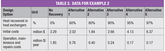
Example 2: Finding the optimum design — thermal energy recovery at a plant preheat train. In this example, the preheating section of a plant is composed of heat exchangers and a furnace located upstream of the reactor. The heat exchangers will transfer heat from the reaction products to the reactants, and the furnace will cover the last heat addition to reach the required reactor inlet temperature. The design team is now trying to select the optimum design (that is, the amount of heat recovered at the heat exchangers that generates the lowest LCC), taking into consideration the limitation that the furnace design duty must be kept above a minimum value for plant startup.
After interaction between process and cost engineers, the team estimates the initial, operations, maintenance and repair costs included in Table 2. Disposal and replacement costs, and residual value are determined not to be significantly different between each alternative, and additional economic benefits are found to be negligible. The design team will perform the evaluation at study periods of 10 years and 20 years, and real discount rates of 10% and 5%.
In this example, to obtain the optimum design, the team needs to calculate the present value of the recurring operations, maintenance and repairs costs by using Equation (4) for each study period and discount rate evaluated, and then obtain the LCC for each option using Equation (1). The results are shown on Table 3.
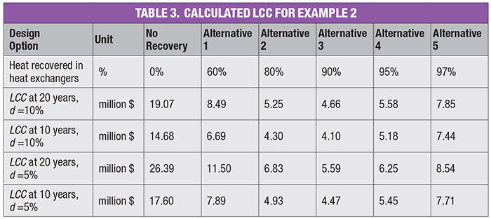
As can be seen in Table 3, Alternative 3 (90% of heat recovered) presents the minimum LCC for this example and is thus the favorable option among those considered in the LCCA. However, the design team may choose to plot the costs of Tables 2 and 3 against the optimized variable (energy recovered in the heat exchangers), as seen in Figure 1.
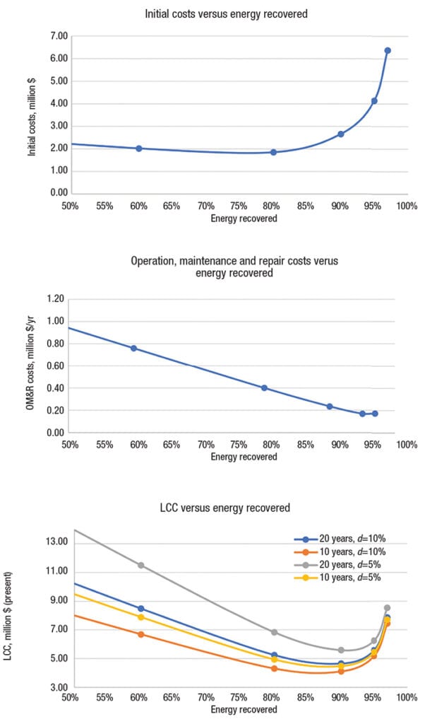
Figure 1. The data and results of Example 2 are plotted in these three graphs
From Figure 1, the following behavior can be observed:
• Initial costs increase exponentially as the efficiency approaches 100%. In this example, the reason for this cost increase lies in the fact that as more energy is recovered in the heat exchangers, the log mean temperature difference becomes smaller, thus requiring larger heat transfer area. this cost increase behavior is exhibited by many other unit operations, such as mass transfer or separation (for example, cost increases significantly when aiming to increase the purity of one product from 90% to 99%, and then to 99.9%).
• Future cost savings are not necessarily linear with increasing efficiency. In this example, each new heat exchanger reduces operation, maintenance and repair costs for the plant in an almost linear manner until a point (near 95% energy recovery), when cost reduction becomes smaller or costs start to increase. in this ex- ample, the additional cost of maintenance to clean the heat exchangers (and to a lesser extent the additional electrical consumption in pumps to overcome pressure losses) outweighs fuel-gas cost savings after this point. this behavior can also be seen in many other cases, as benefits (or in this case, cost reductions) typically follow the law of diminishing marginal returns.
• The LCC plotted against the optimized variable forms a U-shaped curve with a clear optimum. This optimum value is in uenced by the study period, as well as the discount rate. in this example, the optimum value for a 10-year period at a 10% discount rate is near 85% energy recovery, whereas the optimum for a 20-year period at a 5% discount rate is closer to 92% energy recovery. Generally, shorter study periods and higher discount rates favor alternatives with lower initial costs, whereas larger time horizons and lower discount rates favor alter- natives with lower recurring future costs.
LCCA in circular economy
In the previous sections the LCCA has been described and broken down to its most important parts. By this point, we know that there are typically six main components to the lifecycle cost of a project, and that defining them requires close interaction between the project design team (with process engineers having a lead role) and cost engineers at different project phases, and an important amount of forecasting. The multidisciplinary and forward-looking nature of this type of analysis lends itself to the innovation of green solutions.
In today’s economy, there are many aspects to be considered, with the transition toward cleaner energies and processes gaining importance. This transition not only considers moving from fossil fuels to sustainable energies, but brings on new terms such as “circular economy” and “eco-innovation.”
Eco-innovation (EI) is defined as any innovation that leads toward a sustainable, or durable, development [8], while circular economy (CE) is defined as a strategy to close economical loops on a permanently regenerative economy to rethink the lifecycle of a product [9]. In other words, one aims to create new eco-friendly solutions while the other plans for them to come into a full circle and generate profit all around.
As mentioned before, the LCCA is the breakdown of a project in which the best economic and business alternatives throughout a project’s life are studied. The LCCA comes almost naturally to the implementation of both EI and CE, because it is a tool through which alternatives (such as the recycling of parts) can be planned from a very early stage.
Additionally, by creating a broader picture of the project’s life we are enabled to plan and prepare for gains and possible losses from the very beginning. This is applied with the main idea behind eco-innovation to enhance performance through ecotechnologies and enter already existing markets [8], as it provides a sort of plan of action. The LCCA not only aids entrance into the market but gives the innovator an upper hand for the typical “and then what?” questions posed by investors.
This is particularly true for markets where companies are being encouraged to take these new, greener routes [9] in order to reduce environmental impacts. Moreover, closing “loose ends” is an asset to any project as the current market aims to gain competitiveness by minimizing the waste of materials and energy [8] while increasing efficiencies and productivity.
As our world adapts to the new idea and commitment to an environmental transition, and all its new terms and laws, the LCCA plays a key role in determining who will have a competitive advantage in the market.
Acknowledgements
The authors would like to thank Mr. Freddie Sarhan ([email protected]) from Calnetix Technologies, LLC (www.calnetix.com) for providing information that served as a basis for the expander energy-recovery example in this article.
References
1. Bakker, Stefan, “Optimizing the Design-to-Cost Cycle,” Chem.Eng., December 2015, pp. 34–37.
2. Lee Jr., Douglass B., Fundamentals of Lfe-cycle Cost Analysis, Transportation Research Record 1812.1, pp. 203–210, 2002.
3. Nationwide Consulting LLC, “Understanding Life-Cycle Cost Analysis; Why Projects Must Have One,” Nationwide Consulting LLC, 9 Mar. 2018.
4. Chiu, Alfred, Time Value of Money, Chem.Eng., December 2017, pp. 47–49.
5. Association for the Advancement of Cost Engineering (AACE) Recommended Practice 18R-97 “Cost Estimate Classification System – As Applied in Engineering, Procurement, and Construction for the Process Industries” Revision date 2019/03/06.
6. Malta Intelligent Energy Management Agency (MIEMA), “Module 7: Life Cycle Assessment,” Curso: Module 7: Life Cycle Assessment, January 2019.
7. Mearig, Tim, others, “Life Cycle Cost Analysis Handbook,” State of Alaska, Dept. of Education and Early Development, 2018.
8. Commission Européenne. “L’Éco-Innovation, La Clé De La Compétitivité Future De l’Europe.” https://ec.europa.eu/environment/ecoap, 28 April 2020.
9. De Jesus, Ana, et al. “Eco-innovation in the transition to a circular economy: An analytical literature review.” Journal of Cleaner Production, 172, pp. 2,999–3,018, 2008.
Authors
 Sebastiano Giardinella is the vice president and co-owner of the Ecotek group of companies (Bldg. 239, 3rd floor, City of Knowledge, Panama City, Panama / Coral Gables, FL, USA; Phone: +507 64610311; Email: [email protected]). He has experience in feasibility studies, corporate management, project management and process engineering consulting in projects for the chemical and energy industries. He is a project management professional (PMP), has a M.Sc. in renewable energy development from Heriot-Watt University (Scotland, 2014), a Master’s Degree in project management from Universidad Latina de Panamá (Panama, 2009), and a degree in chemical engineering from Universidad Simón Bolívar (Venezuela, 2006). He has written technical publications for Chemical Engineering magazine and international associations, and holds one patent for an energy storage system and method.
 Zabdyk V. Baumeister is a civil engineer graduated from Florida State University (2019). She is currently studying a Master of Ecotechnologies for Sustainability and Environmental Management in Ecole Polytechnique de Paris (Email: [email protected]). She has experience in engineering design for mining and energy industry, as well as in research and development for soil analysis and leachate sewage on landfills.
 Alberto Baumeister is the CEO and co-owner of the Ecotek group of companies (same address as above; Email: [email protected]). He has experience in corporate management, project management, and senior process consulting in engineering projects for the chemical, petrochemical, refining, oil and gas, electrical power generation and agro-industrial industries. He has a Specialization in Environmental Engineering (Gas Effluents Treatment) from the Universidad Miguel de Cervantes (Spain, 2013), a Master’s Diploma in water treatment management from Universidad de León (Spain, 2011), a specialization in management for engineers at Instituto de Estudios Superiores de Administración (Venezuela, 1990), and a degree in chemical engineering from Universidad Metropolitana (Venezuela, 1987), graduating first of his class. He was professor of the Chemical Engineering School at Universidad Metropolitana between 1995 and 2007 and has written several technical publications for Chemical Engineering magazine, academic institutions and international associations.