Light hydrocarbons in storage tanks can vaporize and vent to the atmosphere, creating harmful emissions. An optimized vapor-recovery unit can effectively and economically reduce such emissions
In the chemicals, petroleum refining and natural gas industries, storage vessels are used to contain various liquids, such as condensates, crude oil and produced water. Condensate and crude oil are usually kept in fixed-roof, atmospheric-pressure tanks between production wells and pipelines or truck transportation. In offshore fields, the storage vessels usually contain crude oil and condensate produced from connected wells, or from nearby platforms [1].
In most cases, light hydrocarbons, such as methane, volatile organic compounds (VOCs), natural gas liquids (NGLs) and hazardous air pollutants (HAPs), in the crude oil tend to vaporize and collect within the space between the fixed roof and liquid level of the tank [2]. Ambient temperature changes cause the fluctuation of liquid level in the tank, leading to the escape of vapors into the atmosphere. These escaped vapors cause income losses due to reduction in hydrocarbon volume and changes in the American Petroleum Institute (API) gravity measure of the oil. Apart from potential fire hazards, they also contribute to environmental pollution, because methane (C1) and carbon dioxide (CO 2) are greenhouse gases that contribute to global warming [3].
Flash gases may be flared or vented directly to the atmosphere — the latter results in an environmental emissions impact [4]. Therefore, a commonly accepted option to simultaneously reduce light hydrocarbon emissions and realize significant economic savings is to install vapor-recovery units (VRUs) on storage vessels. VRUs are relatively simple systems that can capture approximately 95% of the light hydrocarbon vapors for sale, or for onsite usage — for instance, as fuel. Ref. 2 reported the generation of savings from recovering light hydrocarbons, while at the same time reducing the volume of HAPs and methane emissions.
For this article, simulation and optimization were performed on a VRU for the recovery of light hydrocarbons. The process parameters that affect profitability were identified and optimized in order to achieve higher profitability for the VRU.
Base-case simulation
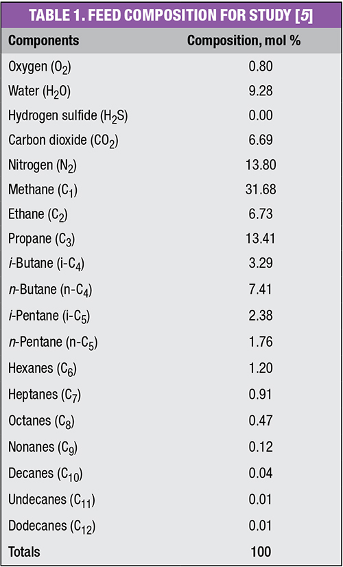 A base-case simulation model (Figure 1) was developed using the commercial process simulation software Aspen Hysys v8.8, using a thermodynamic package employing the Peng-Robinson equation of state, which is frequently used to evaluate natural gas systems in industry. The feedstream composition is taken from a literature case study reported for a floating production storage and offloading (FPSO) unit [5], as shown in Table 1.
As shown in Figure 1, light hydrocarbon feed (Stream 1) that is vented or flared from a storage vessel is fed at atmospheric conditions (1 atm and 40ºC) to a liquid ring compressor. The feed is compressed to a pressure that corresponds to the maximum temperature (150ºC) at the outlet of the compressor (in order to prevent damage to the compressor). The compressed gases then pass through an air cooler (with a pressure drop of 0.3 barg), where ambient air at 35ºC is used for cooling. Next, a suction scrubber (a three-phase separator) is used to separate the gas phase (Stream 4) and aqueous layer (Stream 6) from the product (Stream 5), which is the organic phase.
The separated organic phase in the product stream is delivered into a surge vessel for sale, or for further processing. The aqueous phase in Stream 6, which mostly consists of water, is mixed with the expanded gas (Stream 13) with a small amount of hydrocarbon before entering the heat exchanger (HE) as the cooling medium. Upon exiting the HE, this stream is then flared or vented.
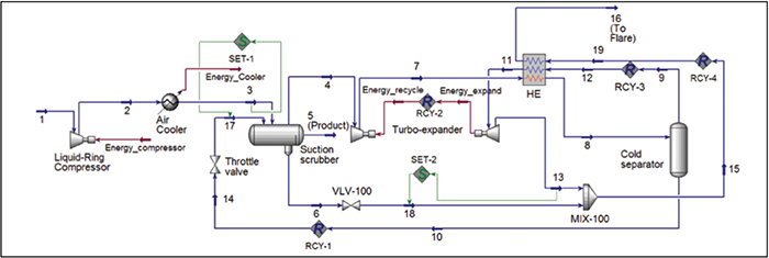
FIGURE 1. The simulation model for this optimization exercise was developed using Aspen HYSYS software
The gas phase from the suction scrubber (Stream 4), which mostly consists of light hydrocarbons and some unwanted gases, is sent to the compressor section of a turbo-expander. The latter is used to convert energy from expanding the high-pressure gases to drive the compressor or generator [6]. The compressed hydrocarbon gases next enter the HE (with a pressure drop of 0.3 barg), which is being cooled to partially condense its hydrocarbon gases. The hydrocarbon gases next enter a cold separator where the unwanted gases are separated and sent to the HE as cooling medium. The unwanted gases, with a pressure of 19 barg, next enter the expander section of the turbo-expander, to recover their pressure. The condensate from the cold separator is recycled to the suction scrubber in order to recover the uncaptured hydrocarbon.
Note that the temperature of the entire system should be maintained in order to prevent icing and hydrate formation in the pipelines. The expanded gas (Stream 13) is the only potential stream where hydrate may be formed. Hence, the pressure of the expanded gas is to be controlled to avoid the expanded gases stream from reaching hydrate formation temperatures. Furthermore, the outlet of the compressor should not reach temperatures higher than 150ºC to avoid damaging the compressor. It is also worth noting that the maximum pressure of the system is to be maintained below 20 barg for safety and maintenance purposes. Within the simulation, two set operation models were used to maintain the pressure of the streams to avoid backflow.
Parametric studies
The purpose of parametric studies is to examine the effect of operating parameters, such as compression ratio (CR) of the liquid ring compressor, temperature at air cooler outlet (Stream 3), pressure of expanded gas (Stream 13) and temperature of Stream 16, on the recovery of hydrocarbon in the product stream. Note that the latter also corresponds to the reduction of greenhouse gases (C1 and CO2).
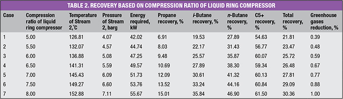
Parameter 1: Compression ratio of liquid ring compressor. In Figure 1, temperature and pressure of the feedstream are set to 40ºC and 0.01 barg (1 atm), respectively. In this study, the liquid ring compressor CR is the parameter being analyzed. The temperature of the air cooler outlet (Stream 3) is kept constant at 50ºC, while that for Stream 16 is kept at 75ºC, and the expanded pressure of Stream 13 is set at 0.4 barg. The simulation results are summarized in Table 2. As shown, the total recovery of hydrocarbon in the product stream increases when the compression ratio is increased. To maximize the recovery of hydrocarbon and yet remain bound to the above-mentioned constraints, the optimum CR should be 7.5, in order to maintain the outlet temperature of the liquid ring compressor lower than 150˚C.
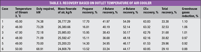
Parameter 2: Temperature at air cooler outlet (Stream 3). For this case, the CR of the liquid ring compressor is set to 7.5, the temperature of Stream 16 is set at 75ºC and the expanded pressure of Stream 13 at 0.4 barg. The temperature of the ambient air, which is used as coolant for the air cooler, is set to 35ºC, to allow a minimum temperature difference (ΔT) of 10ºC. Hence, the lowest exit temperature of Stream 3 is at 45ºC. The simulation results are summarized in Table 3. As shown, the recovery of hydrocarbon is inversely proportional to the increase in temperature. Hence, the lowest temperature of Stream 3 (45ºC) should be chosen as the optimum condition, as it recovers the most hydrocarbon, which also leads to the highest greenhouse gases reduction.
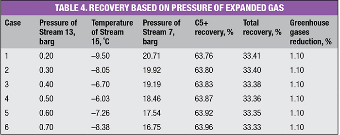
Parameter 3: Expanded pressure at Stream 13.For this case, the compression ratio of the liquid ring compressor is fixed at 7.5, and the temperatures of Streams 3 and 16 are fixed at 45ºC and 75ºC, respectively. Additionally, the pressure of Stream 7 is also observed to ensure the pressure will not go beyond 20 barg. At these conditions, the expanded pressure at Stream 13 is being manipulated, aiming to keep it near atmospheric pressure. Note that the temperature of Stream 15 is being observed because this stream has the highest possibility of forming hydrate.
The results of changing this parameter are summarized in Table 4. Based on these findings, neither C5+ recovery nor greenhouse gases reduction are significantly affected by the expanded pressure of Stream 13. The highest total recovery is observed at 0.2 barg. However, the corresponding temperature of Stream 15 is very low at –9.5ºC, while the pressure of Stream 7 is higher than 20 barg. Hence, a pressure of 0.3 barg at Stream 13 is chosen.
Parameter 4: Temperature of Stream 16.For this case, the CR of the liquid ring compressor is set to 7.5, the temperature of Stream 3 is set to 45ºC and the expanded pressure of Stream 13 is set to 0.3 barg. The temperature of Stream 16 is manipulated to find the optimal temperature that could increase total hydrocarbon recovery, while meeting the minimum approach temperature of 3ºC (by comparing with the temperature of Stream 7). The temperature of Stream 15 is also observed, due to the potential for hydrate formation, as mentioned earlier.
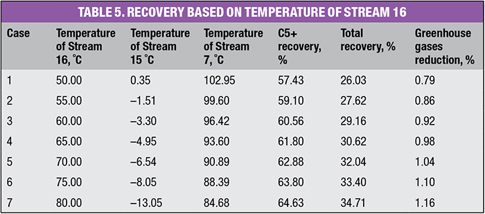
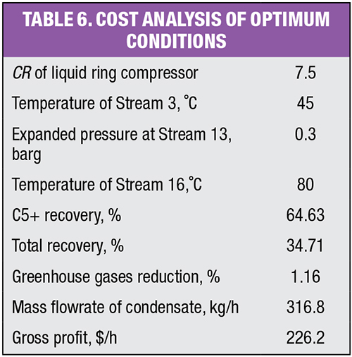
Table 5 shows that the highest total recovery and greenhouse gases reduction is observed at 80ºC. Therefore, this is set as the optimum temperature for Stream 16. After these parametric studies, cost analysis is performed to maximize the profit gain from the VRU. The cost of the condensate recovered from the feed is taken as $50/barrel, while the unit cost of electricity (for compression) is set to $0.02/kWh. Cost analysis results are shown in Table 6.
Hydrate formation study
According to the parametric studies, the pressure of the expanded gas at Stream 13 and the temperature of Stream 16 affect the temperature of Stream 15. In this study, a simulation is done to determine the conditions under which hydrates will form at Stream 15 when Stream 13 is mixed with Stream 6 (which consists mostly of water).
Stream analysis has been carried out using the “envelope” tool in Aspen Hysys in order to identify the conditions for hydrate formation. A hydrate formation graph with pressure versus temperature is shown in Figure 2. Hydrate formation in Stream 15 can occur when there is high pressure and low temperature. In the simulation model, the pressure of the expanded gas in Stream 13 is close to 0.01 barg, which requires very low temperature to form hydrate.
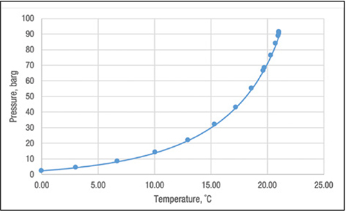
FIGURE 2. This chart shows the conditions where hydrate will form in stream 15
Furthermore, the “hydrate formation” stream analysis tool was also carried out for specific temperatures and pressures to determine the conditions of hydrate formation. The optimum conditions from the four parameter studies were analyzed for hydrate formation. For the optimum conditions of Stream 15 at –13.05ºC and 0.3 barg (see Table 5), hydrate formation does not occur. At 0.3 barg, hydrate formation occurs at a temperature of –18.71ºC; while at –13.05ºC, hydrate will form at 0.75 barg.
From the above analysis, it can be concluded that potential hydrate problems are not significant in this case.
Optimization model
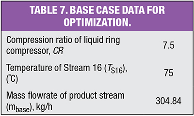 Optimization is next carried out for the VRU, based on the base-case model built earlier. The model was solved using MS Excel Solver, and verified with Lingo commercial software. In this optimization model, the objective was set to maximize the hydrocarbon in the product stream (Δ m prod), while the CR of the liquid ring compressor and the temperature of Stream 16 are the manipulated variables. Note that the temperature of Stream 3 is kept at 45ºC, while the expanded gas pressure (Stream 13) is kept at 8ºC, since those are the optimum conditions that lead to maximum total hydrocarbon recovery. The base-case data for the optimization model are shown in Table 7. The objective of the optimization is given in Equation (1) below:
maxΔmprod = ΔmCR + ΔmS16 + mbase (1)
where ΔmCR is the additional hydrocarbon recovery from the base case (in kg/h) achieved by manipulating the CR value; ΔmS16 is additional hydrocarbon recovery from the base-case (in kg/h) by manipulating the temperature of Stream 16; and mbase is the base case product flowrate of the product stream (304.84 kg/h).
Three scenarios are analyzed in the optimization model. Scenario 1’s goal is to maximize the product flowrate based on the constraints outlined in the base-case section. Scenario 2 explores the possibility of increasing the boundary range of constraint (outlet temperature of the liquid ring compressor), in order to maximize the increment of its gross profit. In Scenario 3, a new constraint is added to reduce the risk of hydrate formation.
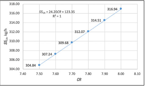
FIGURE 3. This chart displays the relationship between the product stream yield and compression ratio (CR)
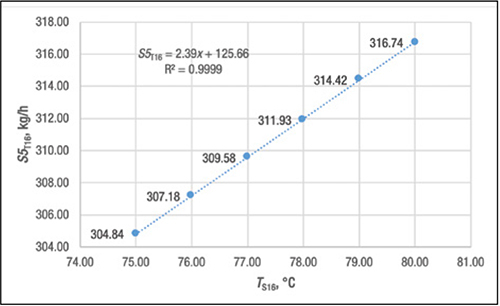
FIGURE 4. The relationship between the product stream yield and the Stream 16 temperature is nearly linear
Scenario 1.To maximize mass flowrate of the product stream (Δmprod), the relationships between ΔmS5 and its manipulating variables (CR and TS16) are first determined. Their relationships are first determined independently. By running the simulation model in Aspen Hysys, the flowrate of the product stream as a result of manipulating the variables is shown in Figures 3 and 4, respectively. As shown in Figures 3 and 4, the relationships of these variables show a linear trend. The linear relations are then deducted from the base values, and result in the revised form that is shown in Equations (2) and (3).
ΔmCR = S5CR – mbase = 24.2 CR — 181.49 (2)
ΔmS16 = S5T16 – mbase = 2.39 TS16 – 179.18 (3)
Additionally, the temperature of Stream 2 ( TS2) is dependent on the compression ratio, as shown in Equation (4). On the other hand, the temperature difference between Streams 16 and 7 (ΔT) is given in Equation (5).
TS2 = 7.21 CR+ 95.23 (4)
ΔT= –0.098( TS16) 2 + 13.44 TS16 – 444.28 (5)
The constraints are given below in boundary Equations (6) and (7):
TS2 ≤ 150°C (6)
ΔT ≥3°C (7)
The objective in Equation (1) is solved, subject to the constraints in Equations (2) through (7), resulting in a product flowrate of 320.8 kg/h. The optimization results were re-simulated and verified with Aspen Hysys. The optimal results for CR(7.6) and TS16 (80.74ºC) obtained from the optimization model are also verified by re-running the simulation model in Aspen Hysys. The difference between the optimization and simulation models is determined as approximately 0.04%, which is negligible.
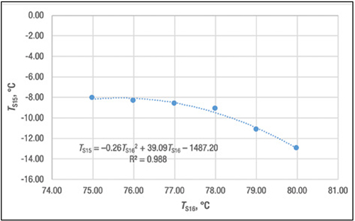
FIGURE 5. The temperatures of Streams 15 and 16 are correlated here
Scenario 2. In this scenario, the objective remains the same as in Scenario 1. However, temperature for Stream 2 ( TS2) is set to be 5ºC above the actual restriction, which is 155ºC. This is because the increase of CR values increases the product mass flowrate of Stream 5 (see Figure 5), which generates higher income. Therefore, a new constraint is added as in Equation (8):
TS2 ≤ 155ºC (8)
Note that all the other constraints remain the same as in Scenario 1. Solving for the objective in Equation (1), subject to the constraints in Equations (2) through (5) and Equations (7) and (8), resulted in a product flowrate of 337.2 kg/h. The optimization results were verified with Aspen Hysys. Re-running the simulation model in Aspen Hysys shows 0.15% difference from the optimization model, which can be neglected.
Scenario 3. In this scenario, the objective is the same as Scenario 1, but a new constraint is added for Stream 15 temperature (TS15) to prevent hydrate formation. Hydrate formation could reduce the hydrocarbon recovery, as well as the profit. Although the hydrate formation study indicated that the formation temperature is much lower at –18.71ºC (0.3 barg), to reduce the risk of hydrate formation, TS15 is set to be higher than –10ºC in Equation (9):
TS15 ≥ –10ºC (9)
Note also that TS15 depends on the Stream 16 temperature (TS16), as shown in Figure 5. The simulation results indicate that their correlation may be given as in Equation (10):
TS15 = –0.26(TS16) 2 + 39.09 TS16 –1,487.2 (10)
Solving the objective in Equation (1), subject to the constraints in Equations (2) through (7) and Equations (9) and (10), yields a product flowrate of 313.2 kg/h. Similar to earlier scenarios, the differences between the Lingo and Hysys models are negligible.
Comparison of results
The results from the base-case model and those from the optimization scenarios are shown in Table 8. As shown, there are increments of gross profit increase for both Scenarios 1 and 2, as compared to the base-case model. Scenario 3, however, shows a decrease in gross profit. The reason for reduced gross profit is due to the additional constraint set for TS15, which causes TS16 to have lower value, and leads to lower gross profit.
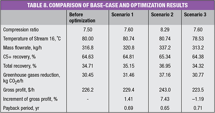
The economic evaluation tool in Aspen Hysys was used to evaluate the economics of the VRU system, resulting in capital cost of $1,263,500 (operating cost is negligible). The payback period of each scenario is shown in Table 8, calculated assuming an annual operating time of 8,000 h. The last row of Table 8 shows that the three scenarios are comparable for their payback period, with Scenario 2 slightly outperforming the others, with the highest greenhouse gas reduction of 37.16 kg of emissions per hour (CO2e/h). Note that the latter is calculated based on the differences of methane and CO2 flowrates in the feed (Stream 1) and Stream 16, which is sent to flare. Note also that methane is generally regarded as a greenhouse gas that is 25 times more powerful than CO2, in terms of global warming potential.
Sensitivity analysis
Sensitivity analysis was next performed to identify the parameters that have significant influence on the gross profit of the project. In the analysis, several parameters, including compression ratio, price of condensate, outlet temperature of Stream 3, temperature of Stream 16 and the price of electricity, were studied to evaluate the gross profit. Each of the parameters is set to have ±20% variation in their values compared to the base-case model.
Based on Figure 6, it can be seen that apart from the price of electricity, all other parameters are very sensitive. The most sensitive parameter is the cooler outlet temperature (Stream 3), which will lead to the biggest difference of gross profit of approximately $100/h. Additionally, the price of condensate will also lead to significant gross profit difference of approximately $90/h.
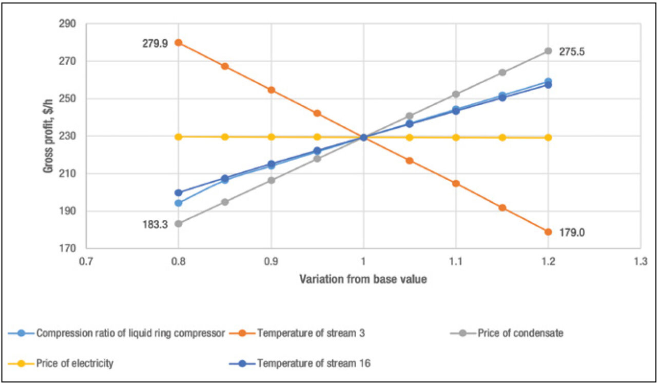
FIGURE 6. Sensitivity analysis shows that most parameters are actually quite sensitive
These analyses confirm that implementation of VRUs on storage vessels reduces pollution while also generating extra profit. The optimization results showed that increased recovery of hydrocarbon leads to increased profit, with a payback period of approximately 0.7 years, coupled with greenhouse gas reduction of more than 30 kg CO2e/h. Sensitivity analysis shows that careful control of Stream 3 temperature is required, because it is the most influential parameter among all those analyzed. ■
References
1. Climate & Clean Air Coalition (CCAC), Technical Guidance Document Number 6: Unstabilized Hydrocarbon Liquid Storage Tanks, 2017.
2. U.S. Environmental Protection Agency, Lessons Learned from Natural Gas STAR Partners, Installing Vapor Recovery Units on Storage Tanks, 2006.
3. Abdel-Aal, H. K., Aggour, M. and Fahim, M. A., “Petroleum and Gas Field Processing,” CRC Press, July 2003.
4. Schneider, G. W., Boyer, B. E. and Goodyear, M. A.. Recovery of flash gas from storage tanks at an offshore production platform using scroll compression technology, Society of Petroleum Engineers — SPE International Conference on Health, Safety and Environment in Oil and Gas Exploration and Production, April 2010.
5. De Vos, D., Duddy, M. and Bronneburg, J.. The problem of inert-gas venting on FPSOs and a straightforward solution, Offshore Technology Conference 2006: New Depths. New Horizons, May 2006.
6. Bloch, H.P., Soares, C., “Turboexpanders and Process Applications,” Gulf Professional Publishing, June 2001.
7. AspenTech, “Aspen HYSYS V8 Highlights, Resources, IT Support For V8,” www.aspentech.com, 2015.
8. Blackwell, B., Vapor recovery systems for tank farms or upstream process separators, Gardner Denver Garo, 2019.
9. Sinnott, R. K. and Towler, G., “Chemical Engineering Design,” Elsevier, 2013.
Authors
 Yik Fu Lim is an industrial instrumentation and control engineer with Taner Industrial Technology Sdn Bhd (Unit B2 & B3, Jalan SP4/1, Seksyen 4, Taman Serdang Perdana, 43300 Seri Kembangan, Selangor, Malaysia; Phone: 6013- 3331928; E-mail: [email protected]). His work involves developing control and instrumentation schemes supporting Industry 4.0 implementation.
 Dominic C. Y. Foo is a professor of process design and integration at the University of Nottingham, Malaysia Campus (Dept. of Chemical and Environmental Engineering, and Center of Excellence for Green Technologies, Broga Road, 43500 Semenyih, Selangor, Malaysia; Phone: +60(3)-8924-8130; Fax: +60(3)-8924-8017; E-mail: [email protected]). He is a professional engineer registered with the Board of Engineer Malaysia. His research includes the development of process integration techniques for resource conservation and production planning. He has published 8 books and over 190 published papers in numerous technical journals, is the editor-in-chief for Process Integration and Optimization for Sustainability and serves on the editorial boards for several journals.
 Mike Boon Lee Ooi is a lead process engineer at NGLTech Sdn Bhd (Suite 8-3, 8th Floor, Wisma UOA II, No 21, Jalan Pinang, 50450 Kuala Lumpur, Malaysia. Phone: +6016-9364888; E-mail: [email protected]). He has 15 years of working experience in oil-and-gas engineering design. His work includes the development of new technologies for condensate-recovery systems (CRS), low-pressure production units (LPPU), separator designs and slug-suppression systems.