Several methods are available for sizing two-phase pressure-relief valves (PRVs). Here, the API 520 homogeneous direct integration method is compared to a potentially simpler alternative that does not require integration
Two-phase pressure-relief valves (PRVs) have been studied by many researchers. Among the many published works on this subject is the American Petroleum Institute (API) Standard 520 on the Sizing, Selection and Installation of Pressure-Relieving Devices. Part 1 of the API 520 standard (9th edition) describes three methods to size two-phase PRVs, which are described in detail in Annex C. The first method is the HDI (homogeneous direct integration) method (section C.2.1), which has wide applicability. The second method is known as the Omega method for two-phase flashing or non-flashing flow (described in section C.2.2). The third is the Omega method for sub-cooled liquid (described in section C.2.3).
This article examines the HDI method and compares it to an easier alternative method, known as HD (homogeneous direct without integration), which is proposed here. The HD method requires less modeling effort than the HDI method and eliminates the need for integration, but the two methods arrive at the same results, as shown in an example calculation included in this article.
HDI versus HD: An overview
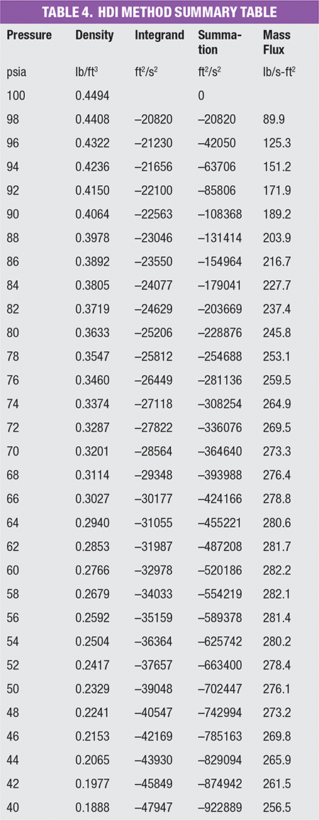
The HDI method involves generating multiple data points over an isentropic range of pressures from the inlet to the discharge of the valve, using a thermodynamic property database. These data are used to evaluate the mass flux integral by direct numerical integration. When this method is put into practice, engineers generally model each isentropic integral through an expander (isentropic flash block) with 100% isentropic efficiency. Depending on the accuracy desired, this may translate into modeling ten or more isentropic flash blocks. Physical properties like pressure and mass density are extracted into a spreadsheet and mass flux is calculated according to the HDI method. The choke point is determined when the mass flux reaches a maximum.
The HDI method requires intensive modeling effort, depending on how close engineers need their result to compare to the actual integration (Figure 1, top). Therefore, an easier method that produces identical mass flux results without integration, would be helpful for engineeers wishing to reduce time and effort required.
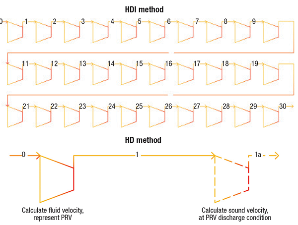
Figure 1. The HDI method (top) requires significant modeling effort, while the HD method without integration (bottom) reduces the modeling effort required in calculating sizes for pressure-relief valves
The HD method without integration proposed here requires only two isentropic flash blocks (Figure 1, bottom), instead of modeling ten or more isentropic flash blocks with the HDI method. For HD, the first isentropic flash block represents the actual PRV, and is used to calculate velocity of the fluid when expanding isentropically from the PRV inlet to the PRV discharge. The second isentropic flash block is used to calculate the velocity of sound at the PRV discharge and it is an imaginary one. If the velocity of fluid is lower than the velocity of sound, it is considered a subsonic pressure relief. The mass flux can be obtained by multiplying the mass density and the velocity of fluid at the PRV discharge condition.
On the other hand, if the velocity of the fluid is greater than the velocity of sound, it is termed a supersonic relief. It is well known that supersonic pressure-relief events cannot occur without a properly designed converging and diverging nozzle. Thus, the maximum fluid velocity in a pressure-relief valve is equal to the velocity of sound. In cases where the velocity of fluid is larger, engineers need to adjust the discharge pressure of the first isentropic flash block so that velocity of fluid equals the velocity of sound. The final adjusted PRV discharge pressure is the choke or critical pressure. The adjustment can be done manually or through a solver in simulation software such as ProMax, an adjuster in HYSYS or a controller in VMGSim. Similarly, the mass flux is calculated by multiplying the mass density and velocity of fluid at this choke (or critical) pressure condition. The required relieving area can then be calculated, using formula C.9 or C.10 in the 9th edition of API 520 Part I.
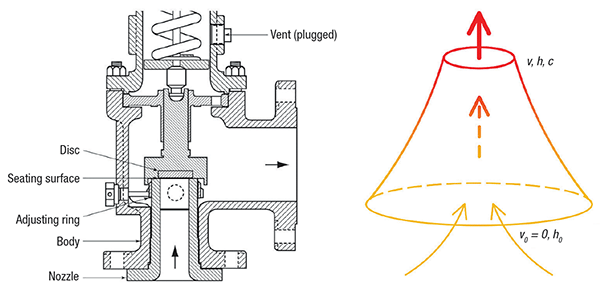
Figure 2. On the left, a diagram of an actual pressure-relief valve is shown, while on the right is a conceptualized nozzle model
Theory behind the HD method
The homogeneous direct (HD) method begins with the same assumptions as those in the HDI method. The most important assumption is that the flow is well mixed — and therefore homogeneous — due to high fluid velocities and a high degree of turbulence found in typical pressure-relief flow. This means that the two-phase mixture can be represented as a “pseudo-single-phase” fluid, with properties that are a suitable average of the individual phase properties.
Fluid velocity calculation. When dealing with pressure-relief flows, it is often convenient to work with properties evaluated at a reference state known as the “stagnation state.” The stagnation state is the state that a flowing fluid would attain if it were decelerated to zero velocity isentropically. Figure 2 illustrates how an actual PRV can be conceptualized into a nozzle model. Compared to the high fluid velocity at the pressure-relief valve throat, the fluid velocity at the relieving condition (PRV inlet) is negligible. Thus,
h 0 = h +( v2 / 2) (1)
After rearranging the formula, the fluid velocity can be calculated in SI units, as follows:
v = √(2 × ( h0 – h)) (2)
Or in U.S. customary (USC) units, using the appropriate conversion factors:
v = √(2 × ( h0 – h) × 2,326/0.30482) (3)
The variables and units for Equations (1) through (7) are described in the nomenclature box above.
Velocity of sound calculation. Velocity of sound can be calculated using the following formulas. In SI units:
c=√( ∆P/∆ρ) (4)
In USC units:
c=√( ∆P/∆ρ × (144 × 32.174)) (5)
Mass flux calculation. Mass flux is mass flowrate per unit area. It can be calculated by multiplying mass density by velocity. For subsonic pressure relief, the equation is as follows:
G = vb × ρb (6)
The equation for a sonic pressure relief is as follows:
G = vt × ρt (7)
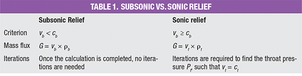
To determine whether the pressure relief is a sub-sonic or sonic relief, first use Pb as the discharge pressure of the first isentropic flash block, and then calculate the velocity of the fluid (vb; Equation (2) or (3)) and velocity of sound (cb; Equation (4) or (5)). If vb < cb, then it should be considered a subsonic relief. If vb = cb, then it is a sonic relief. If vb > cb, then it is a supersonic relief, which can’t happen in a PRV situation. Thus, the discharge pressure needs to increase to Pt, so that vt = ct, and the mass flux should be calculated with properties at the throat condition, instead of the backpressure condition. Sample calculations using this method are shown in the section headed “Sample Calculations using the HD Method” below.
Comparing the methods
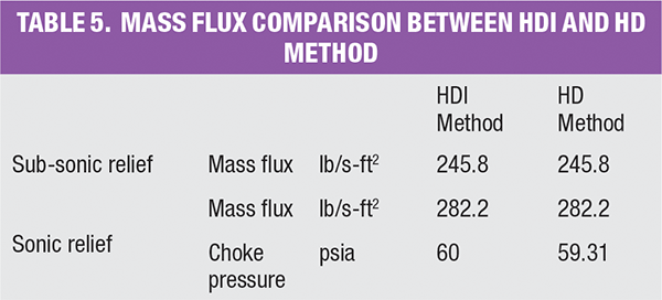
The same example problem can be also solved with HDI method. A summary table of the calculation using the HDI method can be found in the online version of this article. It can be found at the end of this article. Refer to section C.2.1 of API 520 Part I (9th ed.) for the detailed step-by-step calculation. A table summarizing the result from the two methods can be found online. At the backpressure of 80 psia (subsonic relief), both methods yield an identical mass flux of 245.8 lb/s-ft 2. Furthermore, for a sonic relief with a backpressure of 14.7 psia, both methods capture the identical throat pressure at about 60 psia and calculate an identical mass flux of 282.2 lb/s-ft2.
The example clearly shows that the HDI and HD methods produce identical results. But the HD method is generally easier to put into practice by engineers, since it eliminates the integration and requires less modeling effort. In addition, the HD method does not involve any mathematical derivation, such as the mass flux formula in the HDI method. Overall, the HD method is easier and more straightforward for engineers to understand.
Sample calculations using HD method
To illustrate how to properly utilize the HD method to calculate the mass flux of a two-phase pressure relief flow, a sample problem is presented here. ProMax is used as the process simulator and ASME steam is the selected physical property package. Please refer to Figure 1 for the process flow setup. The same exercise can be done directly in an Excel spreadsheet also, if a thermodynamic engine like RefProp is installed on the computer. For this example, the following values are assigned:
Fluid: a steam and water mixture
Relieving (PRV inlet) pressure P0: 100 psia
Relieving steam and water fraction: 50 mol.% each
Relieving flow: 100,000 lb/h
Backpressure Pb scenario 1: 80 psia (subsonic relief)
Backpressure Pb scenario 2: 14.7 psia (sonic relief)
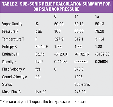
For subsonic relief with a backpressure of 80 psia.
Step 1: Create the first isentropic flash block (expander) to calculate fluid velocity in a process simulator like ProMax. The adiabatic efficiency is 100%. The first isentropic flash block represents the PRV, which goes through an isentropic thermodynamic path. Refer to Figure 1 for additional details.
Step 2: Create the second isentropic flash block (expander) to calculate sound velocity at the PRV discharge condition. The adiabatic efficiency is also 100%. Unlike the first isentropic flash block, which represents the PRV, the second isentropic flash block is an imaginary one that does not physically exist.
Step 3: Specify the relieving conditions as the inlet conditions for the first isentropic flash block. Fluid is H2O, P0 = 100 psia, vapor mole fraction = 50%, mass flow = 100,000 lb/h
Step 4: Specify the discharge pressure of the second isentropic flash block. P1a = 0.99 × P1 (P1 is the first isentropic flash block discharge pressure). This can be done through the “Specifier” function in ProMax, or “Set” in HYSYS and VMGSim.
Step 5: Set the backpressure P b as the outlet pressure of the first isentropic flash block: P1 = Pb = 80 psia
Step 6: Calculate the velocity of fluid using Equation (3) and data from Table 2
v1 = [2 × (–6,123.01 + 6,132.16) × (2,326 / 0.3048 2)] 0.5 = 676.6 ft/s
Step 7: Calculate the velocity of sound using Equation (5) and data from Table 2.
c1 = [(80 – 79.2) / (0.3633 – 0.35984) × 144 × 32.174] 0.5 = 1,036 ft/s
Step 8: Compare v1 and c1. Since v1 < c1, this is a subsonic relief
Step 9: Calculate the mass flux using Equation (6).
G = 676.6 × 0.3633 = 245.8 lb/s-ft 2
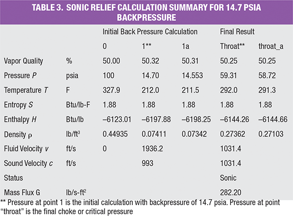
For sonic relief with a backpressure of 14.7 psia
For Steps 1–4, follow the same protocol as in the above subsonic-relief example, then proceed as follows:
Step 5: Set backpressure Pb as the outlet pressure of the first isentropic flash block (P1 = Pb = 14.7 psia)
Step 6: Calculate the velocity of the fluid using Equation (3) and data from Table 3.
vb = [ 2 × (–6,123.01 + 6,197.88) × (2,326 / 0.3048 2)] 0.5 = 1,936.2 ft/s
Step 7: Calculate the velocity of sound using Equation (5) and data from Table 3.
cb = [(14.7 – 14.553) / (0.07411 – 0.07342) × 144 × 32.174] 0.5 = 993 ft/s
Step 8: Compare vb and cb. Since vb > cb, this is a sonic relief, although it looks like a supersonic relief, which is impossible in a PRV pressure-relief situation.
Step 9: Increase the discharge pressure of the first isentropic flash block to P t, then repeat Steps 6 and 7 until v t = c t. This can be done manually or through a solver in the ProMax software, an adjuster in HYSYS or a controller in VMGSim. The final adjusted pressure is the critical pressure, or choke pressure, P t at the throat. At these choke conditions, Pt = 59.31 psia, vt = 1,031.4 ft/s and Þt = 0.27362 lb/ft 3
Step 10: Calculate mass flux using Equation (7). G = 1031.4 × 0.27362 = 282.2 lb/s-ft 2
Editor’s note: For more data on the sample calculations, see Tables below
Edited by Scott Jenkins
References
1. American Petroleum Institute. API Standard 520, “Sizing, Selection, and Installation of Pressure-relieving Devices,” 9th edition, Part 1: Sizing and Selection, July 2014.
2. Darby, R., F.E. Self and V.H. Edwards.,“Properly Size Pressure-Relief Valves for Two-Phase Flow.” Chem. Eng., June 2002, pp. 68–74.
3. Moran, M., and others, “Fundamentals of Engineering Thermodynamics,” John Wiley & Sons, Inc., 8th edition, 2014.
Author
 Guofu Chen is the principal process engineer at Joule Processing LLC (3200 Southwest Freeway, Suite 2390, Houston, TX 77027; Phone (832) 230-9936; Email: [email protected]). He has authored and presented several papers on organic Rankine cycle, natural gas liquid and liquefied natural gas at various conferences. Chen developed rigorous steady-state process models to predict the performance of gas-processing plants with existing unit operations, such as heat exchangers, towers, compressors and control valves. He also utilized dynamic simulation to validate process control, optimize existing plants’ performance and train operators. Chen earned his B.S. in mechanical engineering from Zhejiang University, China. He is both a professional chemical engineer and a professional mechanical engineer in the states of Texas and Louisiana.