This methodology facilitates multifactor testing. However, it comes at a price: a loss in power for detecting effects
The traditional approach to experimentation — often referred to as the “scientific method” — requires changing only one factor at a time (OFAT). Unfortunately, the relatively simplistic OFAT approach falls flat when users are faced with factor interactions, for example, when evaluating the combined impact of time and temperature on exothermic reactions. Because interactions abound in chemical process industries (CPI) operations, the multifactor test matrices that are provided by the design of experiments (DoE) approach appeal greatly to chemical engineers. However, carrying out DoE correctly requires that runs be randomized “whenever possible” [ 1] to counteract the bias that may be introduced by time-related trends, such as aging of feedstocks, decay of catalysts and the like.
But what if complete randomization proves to be so inconvenient that it becomes impossible to run an experiment that is designed in an ideal manner with regard to statistics? In this case, a specialized form of design — called “split plot” — becomes attractive, because of its ability to effectively group hard-to-change (HTC) factors [ 2–3]. A split plot accommodates both HTC factors (for instance, cavities that are being evaluated for their effects on a molding process), and those factors that are considered to be easy to change (ETC; such as the pressure applied to the part being formed).
Split-plot designs originated in the field of agriculture, where experimenters applied one treatment to a large area of land, called a whole plot, and other treatments to smaller areas of land (subplots) within the whole plot. For example, Figure 1 shows two alternative experiments [ 4] that were carried out to evaluate their impact on six varieties of sugar beets (Numbers 1 through 6) that were sown either early (E) versus late (L) in the growing season:
- The top row shows a completely randomized design that was carried out in one field, versus
- The bottom row, which shows the whole plot (a single field) split into two subplots (in this case, parcels with beet crops that were sown early versus sown late)
![FIGURE 1. This figure illustrates a completely randomized experiment (top row) versus one that is split into two subplots (bottom row) [4]](https://www.chemengonline.com/wp-content/uploads/2016/09/19.jpg)
FIGURE 1. This figure illustrates a completely randomized experiment (top row) versus one that is split into two subplots (bottom row) [4]
The split-plot layout made it far sweeter (pun intended) for the sugar beet farmer to sow the seeds according to the proposed grouping, since it is far easier to plant subplots early versus late, rather than doing it in random locations.
Industrial use of the split plot
DoE pioneer George Box developed a clever experiment that led to the discovery of a highly corrosion-resistant coating for steel bars [ 5]. Four different coatings (C1–C4) were tested (which is easy to do) at three different furnace temperatures (which is hard to change), and each experiment was run twice to provide statistical power. The design that Box developed (a split plot) for this experiment is shown in Table 1. Results for relative corrosion resistance — the higher the better — are shown in parentheses. Note the bars being placed at random by position.
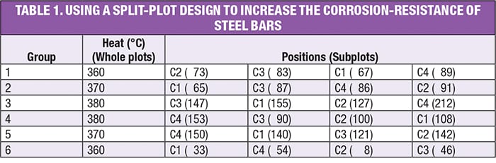
Observe in the layout for this experiment how Box simplified the execution of his experiment: in addition to grouping by temperature (which Box called “heats” in [ 5]), he increased the furnace temperature run-by-run and then decreased it gradually. This was done out of necessity due to the difficulties of heating and cooling a large mass of metal. The saving grace, however, is that, although shortcuts like this may undermine the resulting statistics when they do not account for the restrictions in randomization, the estimates for the effects remain true. Thus, the final results can still be assessed on the basis of subject matter knowledge (in terms of whether they indicate important findings). Nevertheless, if at all possible, it will always be better to randomize levels in the whole plots and, furthermore, reset them (for instance, turn the dial away and then back to the same value) when they have the same value (for example, between Groups 3 and 4 in this design).
In this case, as often happens, the resetting of an HTC factor (temperature) created so much noise in this process that, in a randomized design, it would have overwhelmed the ability to detect the effect of temperature on coating performance. The application of a split plot overcomes this variability by grouping the heats (that is, oven batches), in essence, filtering out the temperature differences.
As shown in Figure 2, the best corrosion resistance occurred for coating C4 at the highest temperature (see the tallest grey tower, located at the back corner). This finding — the result of the two-factor interaction aB between temperature ( a) and coating ( B), achieved significance at p<0.05 (that is, a level of statistical relevance exceeding 95% confidence). The main effect of coating ( B) also emerged as statistically significant.
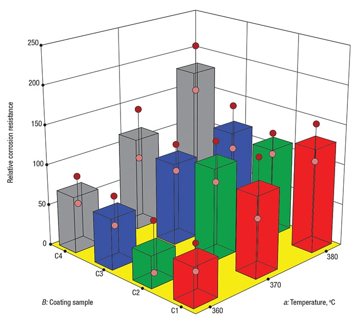
FIGURE 2. In this effects graph, 3-D bars show the impact of temperature (a) versus coating (B) on corrosion resistance — the higher the better
If this experiment had been run in a completely randomized way, the p-values for the coating effect and the coating-temperature interaction would have been roughly 0.4 and 0.85, respectively — that is, not sufficient to be considered statistically significant.
In his work, Box concludes by suggesting that metallurgists try even higher temperatures with the C4 coating while simultaneously working at better controlling the furnace temperature. Furthermore, Box urges the experimenters to work to gain a better understanding of the physiochemical mechanisms causing the corrosion of the steel. This really was the genius of George Box — his matchmaking of empirical modeling tools with his subject-matter expertise.
Some caveats
Split plots essentially combine two experiment designs into one. As a result, they produce both split-plot and whole-plot random errors. For example, the corrosion-resistance design discussed above introduces whole-plot error with each furnace re-set. Such errors arise from potential variation that results from, for instance, operator error in dialing in the temperature, inaccurate calibration, changes in ambient conditions and so forth [ 6]. Meanwhile, subplot errors stem from bad measurements, variation in the distribution of heat within the furnace, differences in the thickness of the steel-bar coatings and more.
This split-error structure creates complications in computing proper p-values for the effects, particularly when departing from a full-factorial, balanced and replicated experiment, such as the corrosion-resistance case. If you really must use this route, be prepared for your DoE software to apply specialized statistical tools that differ from standard analysis.
Furthermore, you cannot expect that doing an experiment more conveniently will not come at a cost — nothing good comes free. The price you pay for taking advantage of split plots is the loss of power to pin down some effects on those factors that are grouped, that is, not completely randomized [ 7].
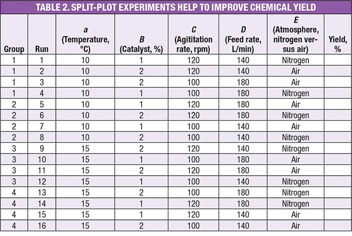
Consider the experiment in Table 2, which tests five factors at two levels, an example taken from a workshop on DoE [ 8]. The factors are:
- a =Temperature, °C
- B = Catalyst, wt.%
- C = Agitation, rpm
- D = Feedrate, L/min
- E = Atmosphere (blanketed by nitrogen or left open to the air)
Note that the first factor is designated by the lower case letter a to distinguish it as being hard to change (HTC), versus the others ( B through E), which are characterized as being easy to change (ETC).
The objective in this experiment is to determine molecular yield, for which normal variation is 2.5% (this is considered “noise”), and a difference of 5% or more is desired to be detected (this is the “signal”). The actual results are not provided here, as that is not relevant to the issues being discussed here. They are matters of experiment design.
Observe in Table 2 how the experiment design groups the runs by temperature ( a) — an HTC factor. This is characteristic of a split-plot design, as opposed to a standard DoE that is completely randomized. The other four factors — those that are ETC — are randomized within each of the four groups.
Based on the user-specified signal-to-noise ratio of 2-to-1, and an HTC/ETC variance ratio of 1 (a standard assumption), the DoE-dedicated software [ 9] that was used to build this design computed the power results that are shown in Table 3.
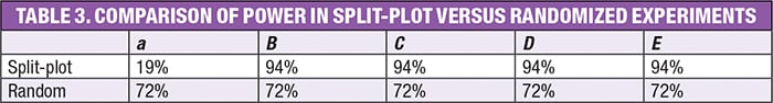
Not surprisingly, the power for the main effect of a (the HTC factor of temperature) drops to a fraction of what it would have been in a completely randomized design — far below the generally accepted level of 80%. On the other hand, the power for the ETC factor effects goes up a bit due to being “protected” from the impact of changing temperature by the grouping.
Furthermore, it turns out that the power for interactions of the HTC with ETCs (that is, the interactions between temperature and catalyst, aB), also comes in higher, for the same reason. Thanks to this bonus, a split-plot design such as this one is a viable alternative to a fully randomized design when a factor such as temperature cannot be easily or quickly changed without creating a big upset in the reaction.
Closing thoughts
Keep the power on HTC factor(s) in mind before settling for a split-plot design. Perhaps grouping HTCs for convenience may not be worth this cost — you would be better off taking the trouble to randomize the whole design. However, for many processes, running any experiment may become impossible if it requires certain factors, such as temperature, to be re-set and equilibrated for each test run; the time and expense to do this becomes prohibitive. These are situations for which a split plot can come to the rescue. — Edited by Suzanne Shelley
References
1. Kleppmann, W., Design of Experiments (DoE): Optimizing Products and Processes Efficiently, Chem. Eng., November 2014, pp. 50–57.
2. Anderson, M.J. and Whitcomb, P.J., “DOE Simplified: Practical Tools for Effective Experimentation,” 3rd ed., Productivity Press, New York, N.Y., 2015, Chapter 11.
3. Anderson, M.J. and Whitcomb, P.J., “RSM Simplified: Optimizing Processes Using Response Surface Methods for Design of Experiments,” 2nd Ed., Productivity Press, Chapter 12, 2016.
4. Cox, D. R., “Planning of Experiments,” John Wiley & Sons, 1958.
5. Box, G.E.P., Split Plot Experiments, Quality Engineering, 8(3), 1996, pp. 515–520.
6. Jones, B., and Nachtsheim, C., Split-Plot Designs: What, Why, and How, Journal of Quality Technology, 41 (4), October 2009, pp. 340–361.
7. Anderson, M.J. and Whitcomb, P.J., Employing Power to ‘Right-Size’ Design of Experiments, ITEA Journal, 35, March 2014, pp. 40–44.
8. Experiment Design Made Easy, Stat-Ease, Inc., Minneapolis. www.statease.com/training/workshops/class-edme.html
9. Design-Expert software, Version 10, Stat-Ease, Inc., Minneapolis, 2016. www.statease.com/software/dx10-trial.html
Author
 Mark J. Anderson is a principal and general manager of Stat-Ease, Inc. (2021 East Hennepin Ave., Suite 480, Minneapolis, MN 55082; Email: mark@statease.com; Phone: 612-746-2032). Prior to joining the firm, he spearheaded an award-winning quality-improvement program for an international manufacturer,generating millions of dollars in profit. Anderson has a diverse array of experience in process development, quality assurance, marketing, purchasing and general management. He is the co-author of two books (Ref. 2 and 3) and has published numerous articles on design of experiments (DOE). He is also a guest lecturer at the University of Minnesota’s Chemical Engineering & Materials Science Department, and Ohio State University’s Fisher College of Business. Anderson is a certified Professional Engineer (PE) in Minnesota, and a Certified Quality Engineer (CQE) in accordance with the American Society of Quality. He holds a B.S.Ch.E. (high distinction) from the University of Minnesota, and an MBA from the University of Minnesota, where he was inducted into Beta Gamma Sigma (the honorary academic society).