 Accurate measurements of exposures to aerosols and dusts by plant personnel can be tricky. Here is some help for determining exposures and addressing uncertainties Uncontrolled aerosols (defined as suspensions of fine solid or liquid particles in gaseous media) in the chemical process industries (CPI) are of significant concern both as explosion hazards and as sources of adverse respiratory-health effects among exposed workers. Events such as the 2008 explosion of airborne and deposited sugar dust at the Imperial Sugar refinery in Port Wentworth, Ga., which killed 16 people and injured 42, are tragic, and conditions leading to this type of explosion are a legitimate cause for alarm. However, sometimes overlooked are the adverse health effects from long-term exposure to airborne contaminants. While the number of early deaths from chronic dust exposures has steadily decreased from a high of nearly 5,500 per year in the early 1970s, airborne dusts still contribute to the illness and early deaths of over 2,000 U.S. workers each year [1]. The combined risks of combustible-dust explosions, and of long-term exposure to airborne dusts make it clear that efforts to measure and control airborne aerosols, including dusts, must continue to ensure workplace safety. Unfortunately, this is not a simple proposition. Barriers remain in determining accurate aerosol concentrations, controlling airborne and fugitive dusts, and knowing what regulations apply to the various sectors of the CPI. This article provides information on how sampling of airborne dust is conducted, how personnel exposures are calculated and how to deal with the uncertainty in those measurements, relative to compliance with governmental regulations.
Personal exposure
Exposure to airborne dust contaminants is determined in nearly every case by measuring the time-weighted average of exposure over the period of a single work shift in the breathing zone of the potentially affected worker. This is referred to as personal sampling for air contaminants. Compliance with legal limits is then determined by comparing the exposure value with the legal permissible exposure limit in a ratio called severity, Y, as follows: Y = (Personal exposure concentration) ÷ (Permissible exposure limit) (1) Once Y is determined, the resulting ratio is adjusted by the sampling and analytical error [SAE; Equations (2) and (3)], and then compared with compliance criteria according to upper and lower 95% confidence limits. SAE is determined from statistical errors of the analytical method(s) used in the laboratory and is combined with the errors resulting from sampling and later handling. Combining errors in this way may result in large SAE values. UCL95% = Y + SAE (2) LCL95% = Y – SAE (3) In Equation (2), UCL is the upper confidence limit and LCL in Equation (3) is the lower confidence limit. Compliance with Occupational Safety and Health Administration (OSHA; Washington, D.C.; www.osha.gov) legal limits is established when the UCL95% is less than one. Non-compliance, along with a possible OSHA citation, is concluded when LCL95% is greater than one. In the condition where LCL is less than one and UCL is greater than one, a possible overexposure is concluded. For exposure concentrations close to the permissible exposure limit, the value of the SAE determines whether an overexposure (or possible overexposure) has occurred. As noted earlier, SAE values can be large, thus interpretation of how errors contribute to the SAE could mean a facility is in non-compliance with federal regulations even though the personal sample is less than the legal limit. Interpretation is not just limited to personal dust exposures. It is the root of the issue for combustible dust safety, as well. LePree [2] outlines the U.S. Federal government’s response to combustible-dust explosions by broadly applying the OSHA General Duty Clause in cases where standards, such as a combustible-dust standard, have yet to be written. This can be confusing for business managers. The presence of clearly written standards — or the intentional absence of them — allows employers to confidently do business knowing they are in compliance with federal and state regulations. In situations where the law is ambiguous and where there is room for broad interpretation, it is arguably “safer” for processors to collect accurate measurements of workplace airborne concentrations using reliable tools and subsequently to control exposures to levels well below the regulatory limits than it is for them to risk being cited for non-compliance and allow unsafe, unhealthy conditions that could lead to explosion or illness. Protecting workers’ health and safety is of paramount importance, but can we go too far in creating overly protective workplaces? In the imaginary world of unlimited resources, the answer would be no. We don’t live in an imaginary world. Resources are indeed limited. Chemical processors feel constant pressure to deliver the highest-quality products, maximize throughput, keep inventories low, protect the health and safety of the entire community, and to have minimal impact on the environment. And these goals are sought within an environment of legal and statistical ambiguity. It is an unenviable position to be in. So what can be done? There are two approaches that can be used to address this challenge. The first is statistical in nature and has immediate application, but it is also overly protective and likely very expensive. The other, engineering design of aerosol samplers, is a longer-term approach but would serve to allow for better characterization of variability so sampling and analytical error of dust exposures would be more tightly controlled. Both approaches are described in the following sections.
Aerosol sampling statistics
Correct and accurate measurement of aerosols in the workplace is dependent on the nature of the material being sampled. Currently, OSHA regulates approximately 500 air contaminants, of which around 10% are aerosols. Respiratory exposure to these materials, and many more that are not regulated, can result in severe adverse health effects or even death. In addition to the health hazard, many of these dusts are known combustion hazards. Table Z-1 of the Toxic and Hazardous Substances, (found in OSHA 29 CFR 1910.1000) is a complete list of federally regulated airborne contaminants and contains legal permissible exposure limits (PEL) for peak, short-term, and eight-hour work-shift exposures. The table lists exposure concentrations in parts per million (ppm) and mass per volume (mg/m3). Generally, gas exposure levels have units in volume-based concentration as ppm, while dust exposures are mass-based concentrations in mg/m3. A number of recognizable materials are found in OSHA’s Table Z-1 including aluminum, malathion, tin and many others. Malathion and tin have PELs for total dust. Aluminum has PELs for total dust and respirable dust. The distinctions between total and respirable dust are important to note because they reflect the location within the lung where disease would be present if exposure were to occur over long periods of time. Total dust refers to exposures that may affect the entire airway, from the nose and mouth down to the alveoli in the gas-exchange region of the lungs. Total dust samplers collect all dust sizes that penetrate past the nose and mouth, which is about 100 micrometers (µm) and smaller. Respirable dust refers to the particulate matter that is of most concern when it penetrates past the upper and middle parts of the airway and then is transported into the gas-exchange region. These dusts are typically less than 10µm in diameter and most are less than 5µm. Conducting personal breathing zone (PBZ) sampling to generate a valid exposure measure requires that the correct sampling protocols be used. For malathion or tin, this would mean sampling for total dust. For aluminum, this could mean sampling for both total and respirable dust concentrations. Instructions for conducting personal sampling are available in the OSHA Technical Manual[3]. Specific sampling protocols for hundreds of materials can be found in the NIOSH Manual of Analytical Methods [4]. Sampling undertaken “in-house” should receive oversight by an industrial hygienist who is certified by the American Board of Industrial Hygiene (ABIH; Lansing, Mich.; www.abih.org). Those who have earned this designation are referred to as Certified Industrial Hygienists (CIHs) and many processors have one or more employed as key members of their environment, safety and health departments.
Example exposure
Suppose the plant safety and health team, in concert with a CIH, has collected full-shift personal breathing-zone samples for two workers over the course of five work shifts. The safety and health (S&H) team thus has five total dust-aluminum measurements to use as indications of each worker’s overall exposure. This is useful for understanding the extent of the exposure experienced by the worker, as well as for predicting what possible exposures may occur in the future. This strategy also allows for the development of a long-term exposure-control strategy and the mitigation of combustible-dust hazards, if present. The example fictitious exposure data collected by the S&H team can be seen in Table 1 for workers with confidential identifiers 094 and 0152. These IDs would be known only to members of the S&H team and possibly to members of company management or human resources dept. In real air-sampling campaigns, the use of identifiers is common and identities are kept in confidence. Note that a large amount of data is collected when conducting air sampling campaigns, some of which is personal, and thus must be protected. Table 1 would represent a small subset of the entire data record. 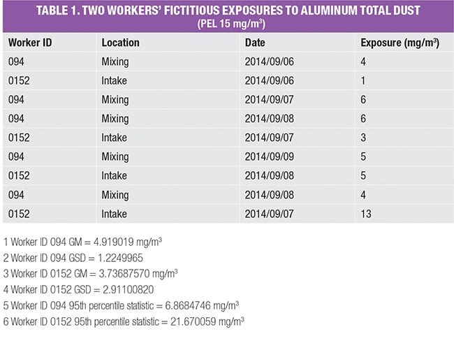 In this case, we treat the personal samples as being lognormally distributed [5–6] and then calculate the geometric mean (GM), geometric standard deviation (GSD) and percentile decision statistics according to Equations (4), (5) and (6), as follows:
 ![]() (4)
(4) ![]() (5) The GM and GSD can be easily calculated by hand. However, IHDataAnalyst software (EASi; www.oesh.com/software.php) can also be used to quickly calculate these values. For the data in Table 1, worker ID 094 has a GM of 4.9 mg/m3 and a GSD of 1.2. Worker ID 0152 has a GM of 3.7 mg/m3 and a GSD of 2.9 [ Editor’s note: for exact values, see footnotes below Table 1 ]. Because the collected air samples are part of the lognormal distribution, with GMs of 4.9 and 3.7, respectively, they accurately represent the data from within those distributions. Note the difference in GSDs between these two groups; one is relatively small, at 1.2, and the other is rather large, at 2.9. A quick look at the raw values for each worker reveals that one is tight (4, 6, 6, 5, 4), while the other has a broader range (1, 6, 5, 13). The tight grouping allows for confident prediction that the next sample taken for worker 094 will likely be close to these values. However, the broader range of the exposure groupings for the second worker opens the door to the possibility that the next value could be very high. This is problematic, as we will soon see.
(5) The GM and GSD can be easily calculated by hand. However, IHDataAnalyst software (EASi; www.oesh.com/software.php) can also be used to quickly calculate these values. For the data in Table 1, worker ID 094 has a GM of 4.9 mg/m3 and a GSD of 1.2. Worker ID 0152 has a GM of 3.7 mg/m3 and a GSD of 2.9 [ Editor’s note: for exact values, see footnotes below Table 1 ]. Because the collected air samples are part of the lognormal distribution, with GMs of 4.9 and 3.7, respectively, they accurately represent the data from within those distributions. Note the difference in GSDs between these two groups; one is relatively small, at 1.2, and the other is rather large, at 2.9. A quick look at the raw values for each worker reveals that one is tight (4, 6, 6, 5, 4), while the other has a broader range (1, 6, 5, 13). The tight grouping allows for confident prediction that the next sample taken for worker 094 will likely be close to these values. However, the broader range of the exposure groupings for the second worker opens the door to the possibility that the next value could be very high. This is problematic, as we will soon see.
Interpreting exposure data
Now that both the GM and GSD for the two workers are known, we can find any value from within the respective distribution by calculating a percentile statistic according to the following: ![]() (6) The product of the geometric mean and geometric standard deviation raised to the power of the z-score for the desired percentile will result in a comparison statistic that can be used to assess risk [5]. We look in the standard normal z-table and see that the 95th percentile corresponds to a z-score of 1.645. Plugging in the GM, GSD and z-score for the grouping of samples for worker 094 gives a value for the 95th percentile statistic of 6.9 mg/m3. We do the same for worker 0152 and get a 95th-percentile statistic of 21.7 mg/m3[ Editor’s note: for exact values, see footnotes for Table 1 ]. These two values are compared to the Exposure Categorization Scheme proposed by the American Industrial Hygiene Association (AIHA) [7] and further developed by Hewett [5] (Table 2).
(6) The product of the geometric mean and geometric standard deviation raised to the power of the z-score for the desired percentile will result in a comparison statistic that can be used to assess risk [5]. We look in the standard normal z-table and see that the 95th percentile corresponds to a z-score of 1.645. Plugging in the GM, GSD and z-score for the grouping of samples for worker 094 gives a value for the 95th percentile statistic of 6.9 mg/m3. We do the same for worker 0152 and get a 95th-percentile statistic of 21.7 mg/m3[ Editor’s note: for exact values, see footnotes for Table 1 ]. These two values are compared to the Exposure Categorization Scheme proposed by the American Industrial Hygiene Association (AIHA) [7] and further developed by Hewett [5] (Table 2). 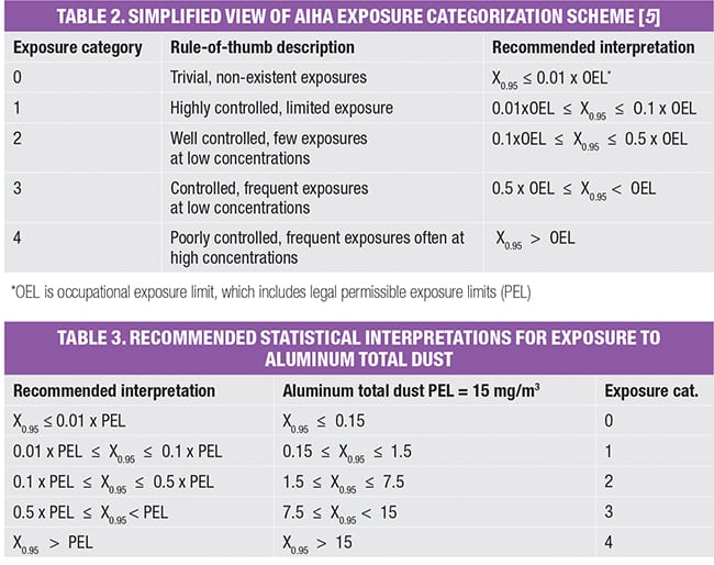 For the current example, we are interested in the PEL for aluminum total dust, which is 15 mg/m3. Applying this value to the recommended statistical interpretation column gives us Table 3. Exposures seen by worker 094 are relatively low and close together, resulting in the 95th percentile decision statistic of 6.9 and thus the exposure category of 2, “well controlled, few exposures at low concentrations,” provides adequate qualification. Those of worker 0152 are low and close together, with one significant exception (at 13). This single high value causes a much higher 95th percentile decision statistic of 21.7 for these lognormally distributed data. This value is well above the PEL of 15, and thus we could say the exposure is “poorly controlled.” It is notable that the lower mean exposure seen by worker 0152 (GM = 3.7) has the higher GSD (2.9), and thus has a much higher 95th percentile statistic. This is because it is associated with the broader range of values. The highest of these, 13 mg/m3, may look like an outlier in comparison with the others in this exposure group. Instead, this value is a true measure of the worker’s exposure to aluminum dust on the day it was collected and serves as an indicator that concentrations of this magnitude do exist. The wide variability of the exposure group sampling measurements for worker 0152 indicate that dust for the associated process is not being controlled. Further, this variability reveals that if this process continues uncontrolled, even higher exposure concentrations could occur. That is, the next sample taken could indicate that the worker is exposed to a concentration of aluminum dust well above 13 mg/m3. We’ve already seen that an SAE of 20% would push this particular sampling result into a legal noncompliance category, indicating that overexposure has occurred. Moving toward the upper end of the distribution of measurements, we would see higher and higher concentrations, all of which would be above the legal limit. The worker could be at risk for adverse health effects and the plant operators would be held responsible for putting the worker in that position. From here, additional exposure categorization work would be valuable, and is recommended. For example, this could include a re-calculation of 95% upper and lower confidence limits, evaluation of the possible use of respiratory protection, adjustments to the ventilation (or other dust-control) systems, collection of additional sampling measurements, and subsequent reassessment of the exposures using a Bayesian approach. As before, such steps should be taken under the watchful guidance of a CIH. Returning to the discussion of the samples in the second worker’s exposure group, the wider variability reveals the presence of uncertainty in the system. The findings do provide enough information to begin taking steps to reduce the exposure concentrations to lower and more consistent values. Most likely this will begin by checking the performance of the ventilation and dust-control systems and then be followed by further investigations, if necessary. In addition to these, there could be other sources of variability and each must be characterized in order to make the system more reliable and predictable. One important source is the fundamental design and performance of aerosol samplers used to collect exposure samples. This aspect of uncertainty determination is taken up in the next section.
Aerosol sampler performance
Multiple samples within an exposure group will each contain multiple sources of variability, which is compounded when we look at the samples over time and space, and from sampler to sampler. Sources of variability buried within the exposure measurement include work rate, work behavior, process being sampled, environmental conditions, pump performance and sampler performance, among others. Aerosol samplers used for sampling the size fraction listed in OSHA Table Z-1, known as total dust, include the 37-mm closed-face sampling cassette, the Institute for Occupational Medicine (IOM) Inhalable Sampler, and the SKC Button sampler. Of these, the first was not designed specifically as an aerosol sampler; rather, it was adapted from the field of water sampling. The latter two were designed in wind tunnels to meet the performance of the inhalability criterion that was established to mimic the concentration by particle size inhaled by a human [8–11]. Subsequent studies have shown that the 37-mm cassette performs like a designed inhalable sampler (like the IOM and SKC button) when wall losses are incorporated into the sample analysis [12–14]. The inhalable fraction expression is given as the following: SI(d) = 0.5(1 + e− 0.06d) (7) where SI(d) is the sampling efficiency for the inhalable fraction and d is the particle diameter. This expression is intended to describe the percentage of particles in the air at specified diameters between 1 and 100µm that will penetrate into the human airway. Adoption of the inhalability criterion has now gone international after early calls to do so [15]. This also includes sampling efficiency prediction for thoracic (50% sampling efficiency cut-set at 10µm) and respirable size fractions (50% cut-set at 4µm), although this article is limited to discussion of the inhalable fraction. These performance metrics for aerosol samplers are now referred to as the CEN/ISO/ACGIH Inhalable Criteria. The criteria were developed in moving air conditions. However, there have been recent calls and studies regarding a calm-air sampling criteria. This makes sense considering that much of the air inhaled by workers really is calm, rather than constantly moving [16, 17]. The CEN/ISO/ACGIH sampling criteria are ideal and protective. These criteria essentially represent the expected average inhalability for humans over the range of particle sizes from 1 to 100µm. The criteria are applicable only to inhalation. That is, when a worker inhales particles and then exhales, the fraction considered for potential illness comes from only the inhalation portion of total respiration. Physiologically, we know that many inhaled particles will be exhaled, however, the current convention is used because aerosol samplers are intended to be operated for continuous inflow, which in turn is a protective approach for assessment of potential illness due to occupational exposure. After all, every human has a different response to exposures and it would be nearly impossible, and certainly financially prohibitive, to continuously monitor every worker, all the time, for any signs or symptoms of illness. Instead, we control exposures to levels well below the PELs and consider any particles that penetrate into the human airway as potential risk candidates for onset of illness. Aerosol samplers, therefore, should collect the size fractions that penetrate into the human airway. Designs of new samplers and redesigns of existing samplers should be based on optimization of performance according to the CEN/ISO/ACGIH Inhalable Criteria for moving air, as well as optimized for a calm-air performance standard. Aerosol samplers have been studied in numerous wind-tunnel and calm-air chamber experiments, but few have been intentionally optimized for agreement with human inhalability. Samplers designed in this way would allow for better characterization of sampling variability and thus reduction in uncertainty when assessing occupational exposures. Edited by Scott Jenkins
References
1. National Institute for Occupational Safety and Health (NIOSH), 2014, “Work Related Lung Disease Surveillance System, All pneumoconioses: Number of deaths, crude and age-adjusted death rates, U.S. residents age 15 and over, 1968–2010,” wwwn.cdc.gov/eworld/Data/All_pneumoconioses_Number_of_deaths_crude_and_age-adjusted_death_rates_US_residents_age_15_and_over_19682010/788, accessed February 2015.
2. LePree, J., “Combustible Dust Safety,” Chem. Eng., May 2013; 120, 5, pp 22–26. 2013.
3. Occupational Safety and Health Administration (OSHA), “OSHA Technical Manual,” 1999, www.osha.gov/dts/osta/otm/otm_toc.html, accessed February 2015.
4. National Institute for Occupational Safety and Health (NIOSH), “NIOSH Manual of Analytical Methods,” 2003, www.cdc.gov/niosh/docs/2003-154/default.html., accessed February 2015.
5. Hewett, P., Logan, P., Mulhausen, J., Ramachandran, G., and Banerjee, S., Rating Exposure Control Using Bayesian Decision Analysis, Journal of Occupational and Environmental Hygiene, 3: pp. 568-581. 2006.
6. Wachter, J. and Bird, A., Applied Quantitative Methods for Occupational Safety and Health, University Readers, pp. 138141. 2011
7. Hawkins, N.C., Norwood, S.K., and Rock, J.C. (eds.), “A Strategy for Occupational Exposure Assessment,” Fairfax, Va.: American Industrial Hygiene Association. 1991
8. Ogden, T. L. and Birkett, J. L., The Human Head as a Dust Sampler, in “Inhaled Particles,” edited by Watson, W.H. 1977.
9. Ogden, T. L. and Birkett, J. L., An Inhalable Dust Sampler for Measuring the Hazard from Total Airborne Particulate, Annals of Occupational Hygiene, Vol. 21, pp. 4150. 1978.
10. Armbruster, L. and Breuer, H., Investigations Into Defining Inhalable Dust, Annals of Occupational Hygiene, Vol. 26, pp. 21. 1982.
11. Mark, D. and Vincent, J. H., A New Sampler for Airborne Total Dust in Workplaces, Annals of Occupational Hygiene, Vol. 30, No. 1, pp. 89102. 1986.
12. Démange, M., Görner, P., Elcabache, J.-M., and Wrobel, R., Field comparison of 37-mm closed-face filter cassettes and IOM samplers, Appl. Occup. Environ. Hyg. Vol. 7, pp. 200208. 2002.
13. Ashley, K. and Harper, M., Analytical Performance Issues: Closed-Face Filter Cassette (CFC) Sampling — Guidance on Procedures for Inclusion of Material Adhering to Internal Sampler Surfaces, Journal of Occupational and Environmental Hygiene, Vol. 10: pp. D29-D33, 2013.
14. Ashley, K. and Harper, M., “NIOSH Manual of Analytical Methods – Consideration of Sampler Wall Deposits,” 2014, www.cdc.gov/niosh/docs/2003-154/cassetteguidance.html, accessed February 2015.
15. Soderholm, S., Proposed International Conventions for Particle Size-Selective Sampling, Annals of Occupational Hygiene, Vol. 33, No. 3, pp. 301320. Correction, 1991, Annals of Occupational Hygiene, Vol. 35, No. 3 pp. 357358. 1989.
16. Lidén, G. and Harper, M., Analytical Performance Criteria: The Need for an International Sampling Convention for Inhalable Dust in Calm Air, Journal of Occupational and Environmental Hygiene, Vol. 3, pp. D94D101. 2006
17. Anthony, T. R. and Anderson, K., An Empirical Model of Human Aspiration in Low Velocity Air Using CFD Investigations, Journal of Occupational and Environmental Hygiene, DOI: 10.1080/15459624.2014.970273. 2014.
Author
 Aaron Bird currently works as the senior training and instructional design manager for the Americas at CD-adapco (21800 Haggerty Road, Suite 300, Northville, MI 48167; Email: aaron.bird@cd-adapco.com; Phone: 248-277-4600). Bird holds a bachelor’s degree in mathematics from Fairmont State College, a master’s degree in industrial hygiene and a Ph.D. in industrial engineering from West Virginia University (Morgantown, W.Va.). He worked at NIOSH in Morgantown during and after receiving his Ph.D. and then joined CD-adapco as an applications engineer, assisting aerospace, aeronautical and automotive customers with multi-physics simulations. Bird then became an assistant professor in the ABET-accredited Oakland University Occupational Safety and Health Program, where he worked until 2013, when he returned to CD-adapco to assume management of their technical training program. Bird is an author of manuscripts on CFD, statistics, and training; is co-author of an undergraduate textbook on quantitative methods for safety and health; and has presented at national and international conferences.