Viscosity, power consumption, commercial availability and lifecycle cost analysis are all important considerations in pump sizing. An automated spreadsheet method helps engineers take those factors into account in centrifugal pump selection
Many aspiring chemical engineers enter industry after university study without sufficient practical knowledge about how to properly size pumps. A number of recent articles provide useful guidelines for sizing and selecting pumps, but these articles focus on certain specific aspects of proper pump sizing, while leaving out others [1–4]. Chemical engineering literature does not fully cover other essential aspects of pump sizing and selection — including the viscosity correction, power consumption, commercial availability and lifecycle cost analysis.
In industrial operations, pumping alone can account for between 25 and 50% of the total energy usage of the process, depending on the application [5]. The initial purchase price of a pump is only a small fraction of the total lifecycle cost. There are situations in which purchasing a less expensive pump actually leads to greater energy-usage costs. This results in a higher lifecycle cost (see Example 1, below).
Without a proper understanding of the pump selection process, engineers cannot effectively make both economic and practical decisions. This article aims to fill in some of the gaps in understanding and provide a straightforward method for pump sizing and selection. Along with this article, we have created a useful Microsoft Excel spreadsheet to assist with centrifugal pump sizing. The automated Excel spreadsheet assists in calculating the key parameters for pump sizing and selection. Since the majority of the pumps used in the chemical process industries (CPI) are centrifugal pumps, this article focuses on that equipment category, rather than the other general classes of pumps, such as rotary and positive displacement pumps.
Example 1. Pump Sizing and Selection
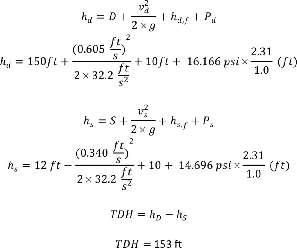
The following is a pump sizing problem to illustrate the calculations in this article. You are told to purchase a pump for your manufacturing facility that will carry water to the top of a tower at your facility. The pump is a centrifugal pump that will need to pump 800 gal/min when in normal operation. Assume BHP is 32 and 16 horsepower for the 3,500-rpm and 2,850-rpm pumps, respectively, for all pump choices in the composite curve. The pump operates for 8,000 h/yr. Assume all of the pumps are viable for your required flowrate. The suction-side pipe and discharge-side pipe diameters are 4 and 3 in., respectively. The suction tank elevation (S) is 12 ft, and the discharge tank elevation (D) is 150 ft. Pressure on the suction side is atmospheric pressure (1 atm = 14.696 psi) and the pressure on the discharge side is 1.1 atm. Assume that both hd,f and hs,f are roughly 10 ft.
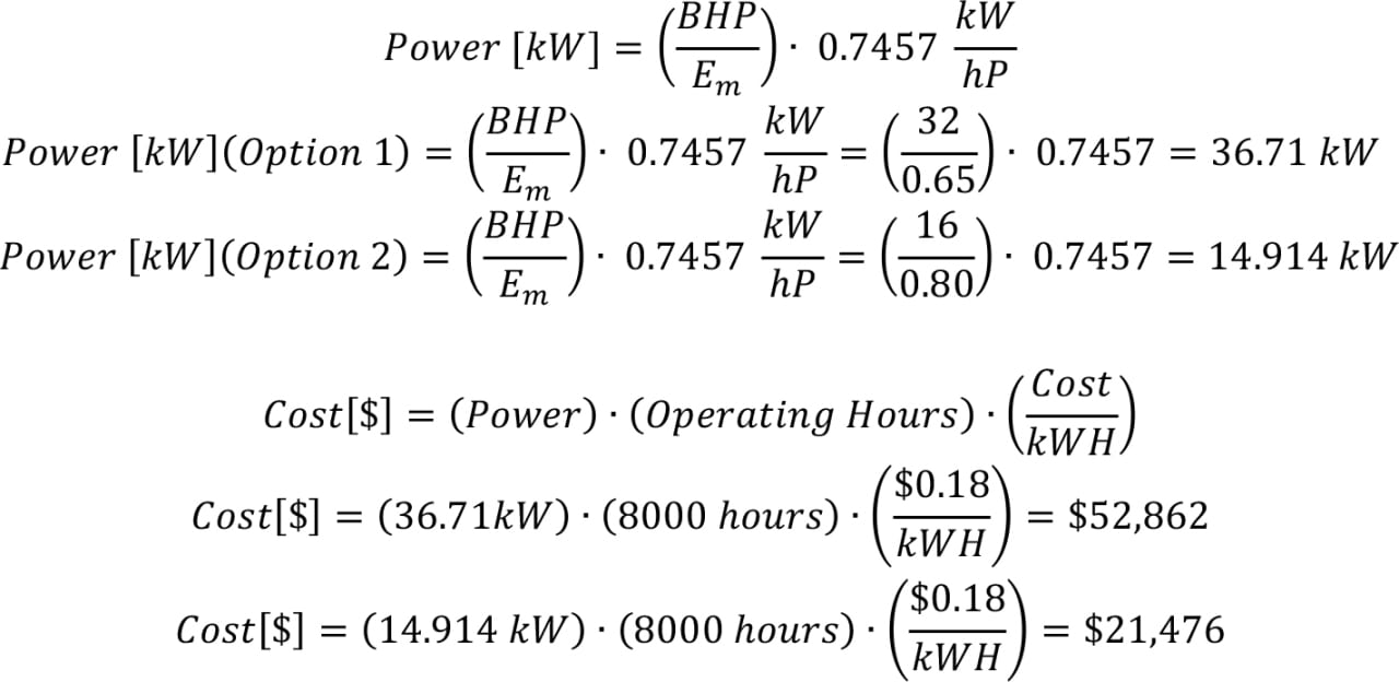
Based on a five-year life, the objective of the problem is to calculate the lifecycle cost to operate each pump (that is, the costs of installation, maintenance and electricity, which is $0.18/kW), and to choose the pump with the lowest lifecycle cost (depreciation is assumed to be negligible for this example). The pump curves in Figure 3 illustrate the following pump options to choose.
Option 1: 4 × 3 – 13 3,500 rpm
Installed cost of pump and motor: $20,000 for 3,500 rpm
Maintenance cost: 10% of installed cost per year
Motor efficiency: 65% (assumed)
Option 2: 4 × 3 – 13 2,850 rpm
Installed cost of pump and motor: $40,000 for 2,850 rpm
Maintenance cost: 8% of installed cost per year
Motor efficiency: 80% (assumed)
Option 3: 4 × 3 – 10 3,500 rpm
Installed cost of pump and motor: $10,000 for 3,500 rpm
Maintenance cost: 10% of installed cost per year
Motor efficiency: 65% (assumed)
Option 4: 4 × 3 – 10 2,850 rpm
Installed cost of pump and motor: $20,000 for 2,850 rpm
Maintenance Cost: 8% of installed cost per year
Motor Efficiency: 80% (assumed)
Solution:
Convert volumetric flow to velocity:
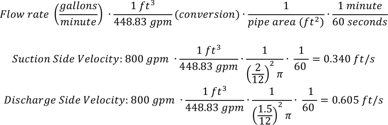
![]()
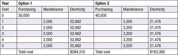
From looking at the TDH and Figure 3, the choice is between Option 1 and Option 2. Notice that most of the TDH comes from the significant elevation difference between the suction and discharge side. Now that two pumps are feasible from the perspective of TDH requirements, you can compare the economics. At first glance, it is tempting to choose Option 1, since the initial investment is significantly lower. Although Option 2 has a higher initial cost, the lifetime cost over five years is dramatically lower. The problem shows that, in selecting a pump, the costs associated with power consumption and maintenance are critical pieces of information for making an informed decision.
Pump sizing overview
The concept of a pumping system is rather simple. The suction side refers to everything before the pump, while the discharge side refers to everything after the pump. Figure 1 illustrates a simplified pumping system. A key parameter in characterizing a pump is the total dynamic head (TDH), which is the difference between the dynamic pressure of the discharge side and the suction side. The dynamic pressure represents the energy required to do the following: (1) to raise the liquid level from the suction tank to the discharge tank; (2) to provide liquid velocity inside both suction and discharge piping; (3) to overcome frictional losses in both suction and discharge piping; and (4) to pump the liquid against the pressure difference between the suction and discharge tanks.
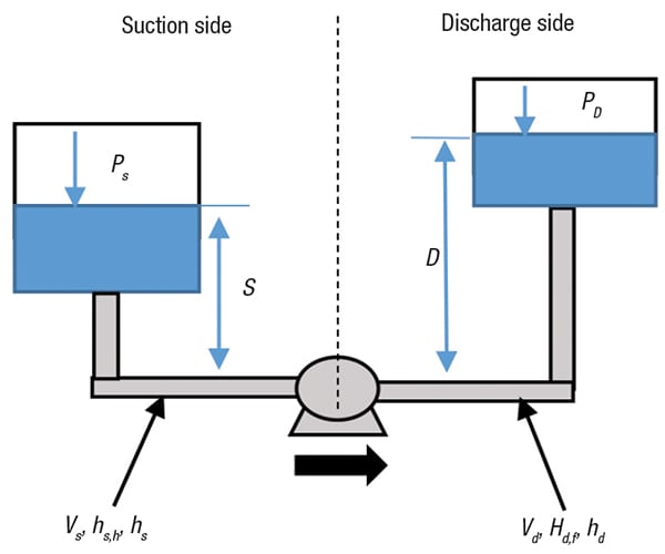
Figure 1. The following components are needed to calculate total dynamic head: suction and discharge elevation; fluid velocity; friction loss and dynamic head; and tank pressure
Six steps to pump sizing. In order to size a pump, engineers need to estimate the temperature, density, viscosity and vapor pressure of the fluid being pumped. Pump sizing can be accomplished in six steps, as follows:
- Find the total dynamic head, which is a function of the four key components of a pumping system, such as the one shown in Figure 1
- Correct for the viscosity of the fluid being pumped, since pump charts and data are given for water with a viscosity of 1 cP. The viscosity of other process fluids can differ dramatically
- Calculate the net positive suction head (NPSH) to select a pump that will not undergo cavitation
- Check the value of suction-specific speed to see if a commercial pump is readily available (see section on suction-specific speed later in this article)
- Check for potentially suitable pumps using a composite performance curve and an individual pump performance curve
- Compare the energy consumption and lifecycle cost of operating the selected pumps
Pump Selection, Example 2
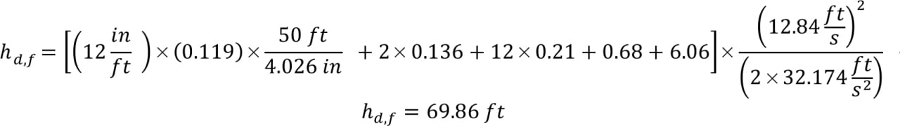
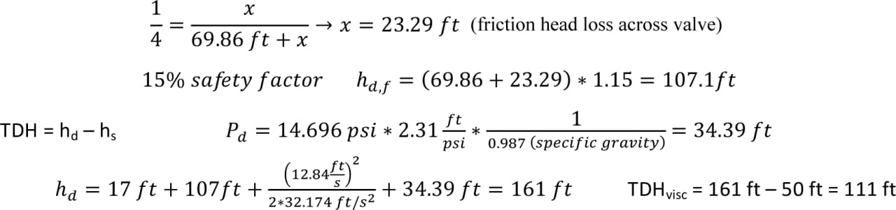
An additional pump selection problem is shown Example 2. For this example, consider a discharge line that is 50 ft schedule 40, 4-in. diameter, with two gate valves, 12 elbows, 1 expander (2–4 in.), a control valve, and a branched tee. The velocity is 12.84 ft/s, Reynolds number is 1,601, and the Darcy friction factor is 0.119. The elevation difference on the discharge side is 17 ft, the total dynamic suction head is 50 ft, and the pressure on the discharge side is 14.696 psi. The objectives in this example are to accomplish the following: 1) Calculate the discharge frictional head loss and total dynamic head; 2) Correct for viscosity of the fluid, which is 300 cP at 125°C; and 3) select an appropriate pump from Figure 3; and 4) Ensure that cavitation is not an issue with the selected pump given the vapor pressure is 13.93 mm Hg and specific gravity is 1.20.
Solution: For choosing the appropriate pump, see Figures 3 and 4. Notice on the pump composite curve, the 4 × 3 – 10 section is very close to the 4 × 3-8G. Both pumps should be analyzed by performing a lifecycle cost analysis using the pump efficiencies from the individual pump performance curves.
![]()
Our NPSHa is much greater than the NPSHr and thus should avoid cavitation under normal operating conditions.
Calculating friction losses
Pumps must overcome the frictional losses of the fluid in order for the fluid to flow in the suction and discharge lines. These frictional losses depend on pipe roughness, valves, fittings, pipe contractions, enlargements, pipe length, flowrate and liquid viscosity.
To calculate the frictional head losses, in feet of liquid being pumped, on the suction (hs,f) and discharge (hd,f) side of the pump, Equation (1) can be used. The same equation can be applied to calculate the frictional losses of the discharge side, but with the appropriate values correlating to the discharge side of the pump.
![]() (1)
(1)
In the equation, fD is the Darcy friction factor, L is the pipe length in feet, I.D. is the inner pipe diameter in inches, v is the average fluid velocity in ft/s, g is the acceleration due to gravity in ft/s 2, ni is the i-th valve, fitting, pipe contraction and enlargement and so on, and ki is the resistance coefficient.
The first term in Equation (1) represents the frictional losses from the fluid flowing through a straight piece of pipe. The second term represents the frictional losses due to valves, fittings, pipe contractions and enlargements. We have provided the values for the typical resistance coefficients and pipe surface roughness from the chemical engineering literature in the Excel spreadsheet discussed in this article.
A control valve follows the widely accepted heuristic of having a friction head loss of 25% of the total calculated friction head loss on the suction or discharge line where the valve is located [4]. An illustration of this solution can be observed in Example 2 on page 40. We also implement the same heuristic within the Excel spreadsheet.
The Darcy friction factor fD can be calculated using the Churchill equation, Equation (2), which is applicable for all values of Reynolds number (Re).
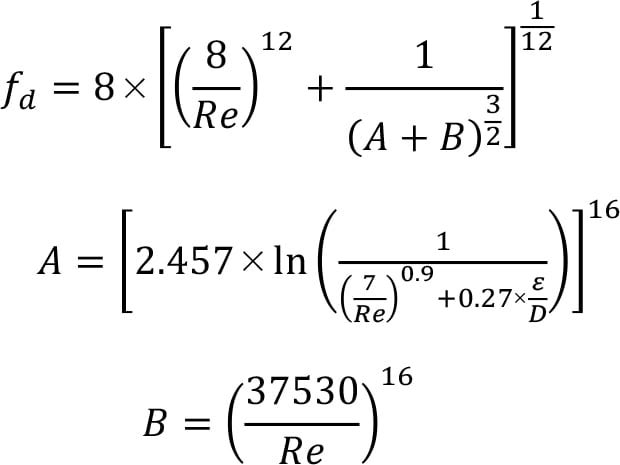 (2)
(2)
In the equation, Re is the Reynolds number and ε/ D is the dimensionless ratio of surface roughness to pipe inner diameter. The equation for the Reynolds number of a circular pipe appears in Equation 3.
![]() (3)
(3)
In the equation, µ is the fluid viscosity, ρ is the fluid density, D is the pipe inner diameter, and v is the average fluid velocity.
A useful heuristic is to add a 15% safety factor to reduce the chance of underestimating the calculated frictional head losses. Sample calculations using these equations appear in the examples within this article.
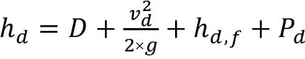
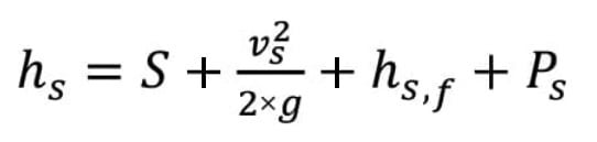
Calculating total dynamic head
To find the total dynamic head, the difference between the discharge velocity head (hD) and the suction velocity head (hs) needs to be calculated.
![]() (4)
(4)
 (5)
(5)
 (6)
(6)
![]() (7)
(7)
The total dynamic head depends on the elevation difference between the discharge tank and suction tank (Figure 1). In Equations (5) and (6), P is the pressure of the suction or discharge side converted to units of length using the specific gravity of the fluid as in Equation (7). The TDH represents the difference between Equations (5) and (6), in which users actually add together the velocity head and the frictional head loss for both the suction and discharge sides of the pump.
Net positive suction head
NPSH is used in the determination of whether the liquid on the suction side of the selected pump will vaporize at the pumping temperature, thus causing cavitation and rendering the pump inoperable. NPSH varies with impeller speed and flowrate.
![]() (8)
(8)
To prevent cavitation in a pumping system, NPSH a should be at least 3 ft above the required NPSH value (denoted by NPSHr) read from the pump curve for the given TDH and pumping rate.
![]() (9)
(9)
Based on Equation (8), there are several ways to increase the NPSHa to make a pumping system feasible. They include the following:
Raise the liquid level in the suction tank (increasing the S term); Lowering the pump location (increasing the S term); Reducing the frictional loss on the suction side (by reducing suction side velocity or pipe length); Pressurizing the suction tank (increase Ps); and Lower vapor pressure by reducing pumping temperature (reduce Pvp).
Viscosity and pump sizing
Viscosity correction is often overlooked in pump sizing by new engineers. As stated previously, all pump curves are drawn for water with a viscosity of 1 cP. Therefore, we need to pay attention to viscosity corrections to pump performance. The Durion Co. Inc., now a part of Flowserve Corp. (Irving, Tex.; www.flowserve.com), has released a simple graphical approach. Head and capacity are not noticeably changed by viscosity below 4.3 cP at pumping temperature. Pump efficiency is reduced when handling liquids with viscosity over 4.3 cP at pumping temperature. Using a fluid with a higher or lower viscosity compared to water changes the dynamics of the centrifugal pump. Power consumption increases rapidly with a viscosity increase because of reduced efficiency. In order to select a pump from standard performance curves, it is necessary to apply correction factors to determine the equivalent pumping rate and total dynamic head for water before reading the pump curves.
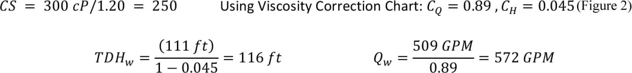
The graphical approach utilizes straight lines to determine simple correction factors for the horsepower, capacity and total dynamic head. First, convert the viscosity units to centistokes (CS) by dividing the centipoise (cP) value by the specific gravity. Referring to Figure 2, start by drawing a straight line from the calculated total dynamic head (A) to the flowrate (B). Then, draw a straight line from the intersection on line C through the known viscosity in centistokes (D) until reaching line E. From line E, one can read the correction factor for break horsepower (Chp). From the intersection on line E, draw a line through point F to line G, where the correction factors for flowrate ( CQ) and total dynamic head ( CH) can be read. We have automated this process in the Excel spreadsheet.
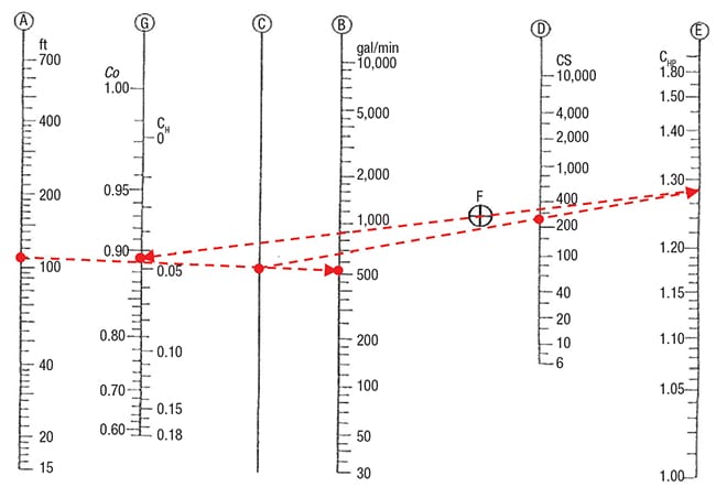
Figure 2. Shown here is a viscosity correction chart. The red dashed line corresponds to Example 2 on p. 40
After obtaining the correction factors, Equations (9), (10) and (11) can be used to correct brake horsepower (BHP) capacity and total dynamic head (TDH). Specifically, input the values for the viscous liquid, use the correction factors read from the chart, and calculate the equivalent water values (especially TDHwater and Qwater) for use in reading pump curves. In Equation (10), assume that the water capacity is at the best efficiency point.
![]() (9)
(9)
![]() (10)
(10)
![]() (11)
(11)
Pump curves
Figure 3 shows a pump composite curve from Griswold Pump Co. (Grand Terrace, Calif.; www.psgdover.com/griswold). Use the pump composite curves to select an appropriate pump for the viscosity-corrected TDH and pumping capacity. The y-axis of the graph is the equivalent water TDH. The x-axis of the graph is the equivalent water volumetric flowrate. Figure 3 has multiple shaded sections, with each corresponding to a different-sized pump. In the individual sections, the pumps are specified by the suction pipe diameter, discharge pipe diameter, and impeller size (4 × 3 – 8G for our selected pump in Example 2). Remember that the larger pipe diameter is always the suction side. For this pump composite curve, there are two x-axes for different impeller speeds. Notice that the two red points both correspond to 570 gal/min of flow and 110 ft of TDH for the different impeller speeds (2,850 and 3,500 rpm). The point that corresponds to this TDH and flowrate may not be the pump that is ultimately selected. For example, if the point is close to the boundary, engineers would need to move vertically up on the composite curve and choose a pump with a larger impeller size (4 × 3 – 10 versus 4 × 3 – 8G). It is very important to always compare the lifecycle cost for the different pumps (see Example 1).
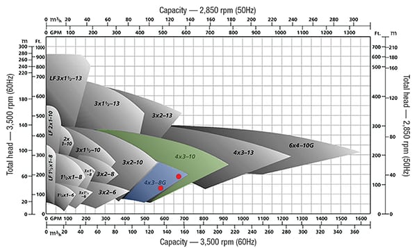
Figure 3. These pump composite curves show the options for Examples 1 and 2
After looking at the pump composite curve and selecting potential pumps, the next step is to look at the individual pump performance curves to obtain the pump efficiency, NPSHr, and impeller size. Figure 4 is an example of an individual pump performance curve. The required NPSH is located at the bottom of this figure, separate from the rest of the performance curve. Keep in mind that not all pump curves are the same and vary by manufacturer. In Figure 4, the blue curve is for an 8-in. impeller diameter. The green curve is for a pump efficiency of 64% and the red curve is for 30 BHP. In most pump curves, engineers could not read the BHP accurately; so instead, we recommend calculating the BHP manually using the pump efficiency according to Equation (12) below.
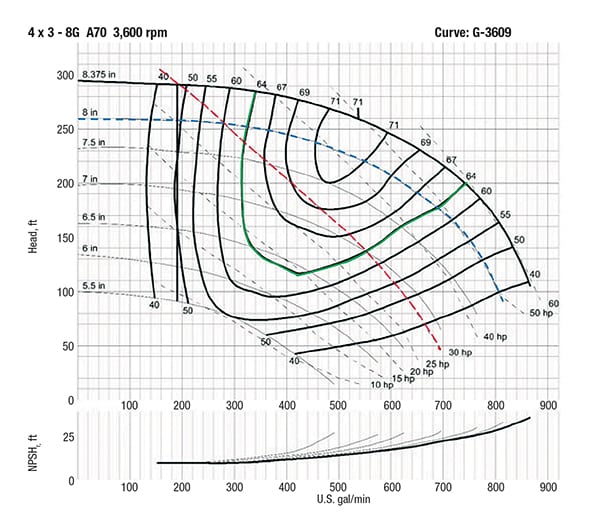
Figure 4. This individual pump performance illustrates Example 2, p. 40
Power and efficiency
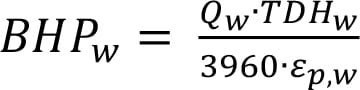
Brake horsepower (BHP) is the actual horsepower delivered to the pump shaft. To find the BHP for a viscous liquid (BHPvis), use Equation (9), after calculating the break horsepower for the equivalent water values (BHPw, TDHwater and Qwater) and efficiency (ξ p,w) from the pump curve using Equation (12).
 (12)
(12)
To determine the electricity cost for operating the pump, use Equations (13), (14) and (15). Equation (13) converts the BHP of your pump to the input power or electricity consumption. Determining the power consumption involves the motor efficiency (Em), which can be obtained from the vendor or estimated from the BHP using the Peter and Timmerhaus correlation, Equation (15) [6].
![]() (13)
(13)
![]() (14)
(14)
![]() (15)
(15)
For an effective cost analysis, estimate the operating hours for an entire year to obtain an electricity cost for one year. Then estimate the lifetime of the pump, how often it needs to be repaired or replaced, and the associated costs. Also, engineers need to contact the pump vendor and ask for a quote on the pump to get an initial cost. This information can be used to perform a simple lifecycle analysis. Consult Example 1 to see how to do this analysis.
Suction specific speed
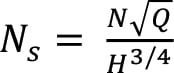
The specific speed is a useful index to help get a general idea of the type of pump to be chosen. All pumps can be broadly classified with a “dimensional” number, as shown in Equation (16).
 (16)
(16)
In Equation (16), N (rpm) is the actual pump rotating speed, Q (gal/min) is the pumping capacity, and H (ft) is the total head at the best efficiency point, corresponding to speed N and capacity Q. Suction specific speed (Ns, rpm) values — obtained by substituting NPSHa for H — of less than 8,500 rpm are typical for commercially available pumps [7]. Specific speed values between 8,500 and 12,000 rpm would likely have to be specially ordered from a pump manufacturer, and values greater than 12,000 rpm are typically not available at all [7].
As defined here, the specific speed represents the pump rotating speed (in rpm) at which a theoretical pump that is geometrically similar to the actual pump would run at its best efficiency to deliver a proportional flowrate.
Automated Excel spreadsheet
The main goal in developing the Excel spreadsheet is to find the total dynamic head to use in reading a pump curve. It can be downloaded at the following URL: http://www.che.vt.edu/Liu-2013/Home.php . The Excel file is broken up into several sheets to allow the user to tackle the sizing of their pump in a series of logical steps. Sheet 1 consists of user inputs and the main outputs of the Excel program (Figure 6). Sheet 2 provides a quick method to calculate the vapor pressure of a fluid using the Antoine equation. In Sheet 2, several variables for the Antoine equation are included for convenience, but the parameters for other fluids not included in the spreadsheet can be readily found in the literature. Sheet 3 is included for finding the friction losses in the pumping system. Inside Sheet 3 are useful tables for summing the typical resistance coefficients for the valve, fitting, contractions and enlargements, and so on, and determining the relative roughness of the piping.
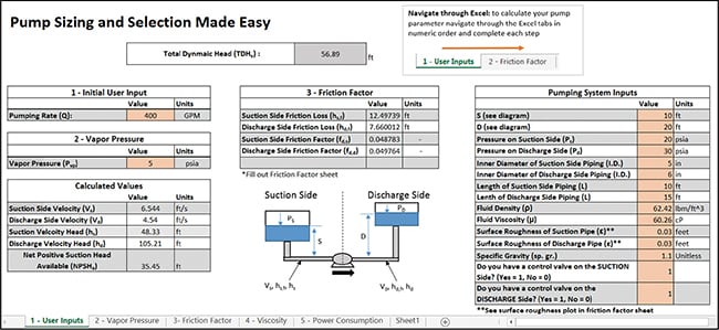
Figure 5. This shows the home screen of the automated Excel spreadsheet. It can be downloaded at this URL: http://design.che.vt.edu/
To perform the viscosity correction, input TDH, flowrate and viscosity (in centistokes) into Sheet 4. Then, input the correction factors from the viscosity correction chart into the appropriate cell in Sheet 4. This Excel spreadsheet uniquely draws the lines on the diagram automatically based in the user’s input. In Sheet 5, power consumption can be found and will provide the annual utility cost of the pump under consideration, as a function of both the yearly operating hours and local electricity cost. n
Edited by Scott Jenkins
Acknowledgements
We would like to thank Flowserve Corp. for allowing us to use their viscosity correction chart. For more information about Flowserve, please visit www.flowserve.com. We would also like to thank Griswold Pumps for allowing us to use their pump curves and pump information to create useful real-world examples. For more information about Griswold Pumps, please visit www.griswoldpump.com. In addition, we would like to thank the Hydraulic Institute (Parsippany, N.J.) for the use of their friction factor correlations in our Excel Spreadsheet. For more information about the Hydraulic Institute, please visit pumps.org.
References
1. Moran, Sean; Pump Sizing: Bridging the Gap between Theory and Practice, Chemical Engineering Progress, pp. 38–44, Dec., 2016.
2. Fernandez, K., Pydrowski, B., Schiller, D. and Smith, M.; Understand the Basics of Centrifugal Pump Operation, Chemical Engineering Progress, pp. 52–56, May, 2002.
3. Kelly, J. Howard; Understand the Fundamentals of Centrifugal, Chemical Engineering Progress, pp. 22–28, October 2010.
4. Raza, Asif; Sizing, Specifying and Selecting Centrifugal Pumps, Chem. Eng., pp. 43–47, February 2013.
5. Pump Life Cycle Costs: A Guide to LCC Analysis for Pumping Systems: Executive Summary. Washington, DC: Office of Industrial Technologies, Energy Efficiency and Renewable Energy, U.S. Dept. of Energy, 2001.
6. Peters, Max., Klaus, Timmerhaus, and West, Ronald, “Plant Design and Economics for Chemical Engineers,” 5th ed. McGraw Hill., New York, p. 516, 2003.
7. Dean Brothers Pumps Inc., Net Positive Suction Head and the use of Suction Specific Speed to Avoid Cavitation, Pump Talk, Indianapolis, Ind., 1982.
Authors
 Joseph “Joey” Sarver is currently pursuing a M.S. degree in chemical engineering at the Virginia Polytechnic Institute and State University (Virginia Tech; Blacksburg, Va.). Previously, he was a post-bachelor research assistant at Oak Ridge National Laboratory (ORNL) through the Oak Ridge Institute for Science and Education developing fabrication methods for organic spintronics using conjugated polymeric materials. He also worked as a co-op student for the United States Gypsum Corp. as a project engineer in the paper division. As an undergraduate, Sarver was actively involved in research at the Virginia Tech Supercritical Fluids laboratories under Erdogan Kiran. His research awards include recognition at the 2016 AIChE international conference for gradient foaming of polymers in supercritical carbon dioxide.
 Blake P. Finkenauer is a first-year Ph.D. candidate in chemical engineering at Purdue University who holds a B.S.Ch.E. degree from Virginia Polytechnic Institute and State University (Phone: 757-696-2462; Email: bfinkena@purdue.edu or bfink757@vt.edu). He has worked as a co-op at the DuPont Spruance Plant in Nomex Process Control and in Polyaramid Research and Development. He also worked at NASA Langley Research Center as an intern in the Langley Aerospace Research Student Scholar (LARSS) Program. As a student at Virginia Tech, Finkenauer conducted undergraduate research in processing thermotropic liquid crystalline polymers under Donald Baird. For his senior design project, he worked with a team of three students for BAE Systems. Finkenauer received numerous awards for his academic achievements, including the AIChE Donald F. Othmer Sophomore Academic Excellence Award, ACS James Lewis Howe Award, and a Ross Fellowship.
 Y. A. Liu is an Alumni Distinguished Professor and the Frank C. Vilbrandt Endowed Professor of Chemical Engineering at Virginia Polytechnic Institute and State University (Virginia Tech; Blacksburg, VA 24061; Phone: 540-231-7800; Email: design@vt.edu). Over the past 30 years, Liu has taught hands-on training courses on energy and water savings, computer-aided design and advanced process control to over 7,000 practicing engineers in the U.S., China and Taiwan. He served as a senior advisor to Sinopec from 2001 to 2015, and to PetroChina since 2016. He has taught design courses to graduating seniors in chemical engineering since 1982, for which pump sizing and selection is a course topic. He is a recipient of the George Westinghouse Award and Fred Merryfield Design Award from the American Society for Engineering Education, the Outstanding Faculty Award from the Virginia’s governor, and the National Friendship Award from the China’s premier. In 2015, he received Virginia Professor of the Year award from the highly selective U.S. Professors of the Year program, sponsored by the Carnegie Foundation for the Advancement of Teaching and the Council for Advancement and Support of Education.
Note from Editors: For an addendum to this article, see https://www.chemengonline.com/addendum-to-pump-sizing-and-selection-made-easy/