Understanding the implications of adiabatic and isothermal flow assumptions is necessary to have confidence in when to use such assumptions
Every engineer uses assumptions because every analysis has an overabundance of variables to consider. Often, there are just too many to analyze and simplifications are made to eliminate variables or create more relationships between them. The decision of what assumptions to make rests on the engineer’s shoulders. Even beyond making a problem solvable, engineers build assumptions into their analyses to make the math easier and faster. Although a problem may be technically solvable, there is value in simplifying the problem further. After all, exact answers do not exist in engineering.
When analyzing something as complex as gas flow through pipes, the math becomes daunting to say the least. Hydraulic modeling of liquid and gas systems are worlds apart, simply because gases have variable density, while liquids do not. (This may not sound like a huge difference, but open a compressible flow textbook, and you will quickly change your mind.)
With all the intricate considerations of compressible flow, heat transfer complicates the situation exponentially. Yet, without analyzing heat transfer, the system model may deviate far from reality. Flow behavior, among other things, relies heavily on temperature. This leaves engineers with a dilemma and often pushes them to simplify their operating conditions with assumptions to make the math easier. Two common assumptions in gas-handling processes are (1) adiabatic flow and (2) isothermal flow. The derivations, implications and outcomes of each assumption need to be understood before an engineer puts confidence in them.
System and boundaries
In any thermodynamic study, defining the system and its boundaries is fundamental. Heat transfer inherently implies energy is transmitted from one point in space to another, thus, crossing some boundary. Similar to defining a reference point in physics, defining the system and boundaries is up to the engineer, as there is technically no “correct” definition. (That is not to say some choices are not better than others.) The boundaries encompass the system. Everything outside the boundaries is considered the surroundings. Once the system and boundaries are defined, analysis is to be done keeping those definitions constant.
In this case, the system is defined as a piping network, where the boundaries contain the pipes and insulation but exclude any upstream and downstream energy-adding components (such as compressors or heat exchangers). In this way, only heat transfer with the surroundings is considered, and work is excluded from the energy balance. A simplified example of a single pipe is shown in Figure 1. The boundaries are represented by the dotted red line, and the system is the enclosed pipe.

Figure 1. Shown here is a hypothetical methane-transfer system. Methane enters at pressure (P) 300 psia (20.5 bars) and 100°F (38°C), with a flowrate (Q) of 5,000 scfm (8,500 scmh). The surrounding air is 60°F (16°C) with low wind at 5 ft/s (1.5 m/s). The system boundaries are represented by the dotted red line. The system is the enclosed pipe [1]
To help solidify the discussed concepts, a hypothetical methane-transport system serves as a tangible example. The system conditions are described in Figure 1. Other properties, such as pipe length, diameter, and insulation thickness, are modified throughout the discussion to analyze the applicability of adiabatic and isothermal flow. However, the inlet conditions, ambient temperature, fluid-mass flowrate and pipe diameter remain constant.
This discussion is focused on steady-state flow systems. Any energy that enters the system must leave, but it may do so as a different form. The full energy balance includes five main components: heat, work, energy from fluid flow in, energy from fluid flow out, and energy accumulation. Right off the bat, both work and energy accumulation are eliminated. Subsequent analyses require looking at the energy balance and determining what does and does not apply. Setting up the problem before anything else is essential.
Even a seemingly simple system like this has complex behavior. Unlike incompressible flow, compressible flow cannot assume a linear pressure profile. Proper analysis requires the “system” to really be a series of infinitely short segments along the length of the pipes. In this way, a typical property difference (represented by a Greek “delta”) found in the incompressible Bernoulli equation becomes a true differential.
Analytical solutions prove difficult to find, so modeling usually requires numerical methods to decide the size of these discrete sections. This article’s discussion revolves around the whole system to display heat transfer concepts, but through modeling software, this system was broken into many pieces to obtain smooth property profiles. It is no wonder engineers pursue ways to simplify the math.
The two most common simplifying assumptions for flow in gas piping systems are to assume adiabatic or isothermal flow. As mentioned, there is no getting out of heat transfer analysis with compressible flow. Gases follow an equation of state, which means the temperature helps determine the volume and pressure of the system. They are coupled together such that heat transfer cannot be ignored.
Adiabatic flow
The term “adiabatic” means no heat is transferred between the system and its surroundings. In piping systems, adiabatic flow means no heat energy crosses that boundary between the system and surroundings. This approximation is applicable in systems with very slow heat transfer with the surroundings. For instance, systems with thick insulation around the pipes and relatively short pipe lengths are good candidates for this assumption.
Adiabatic systems enable the energy balance to completely ignore heat, so the balance boils down to energy internal to the pipes. The gas flowing into and out of our system boundary contains all the energy. The internal gas flow includes kinetic energy and enthalpy. Potential energy is neglected because the system inlet and outlet elevations are equal.
The combination of kinetic energy and enthalpy must be equal for flow entering and exiting the system. If one of the terms decreases at the exit, then the other must increase to maintain the balance. Kinetic energy tends to increase down the pipe, and enthalpy decreases. Velocity increases down the pipe as pressure decreases. Kinetic energy is a function of velocity, so that is why kinetic energy increases.
Enthalpy then decreases to balance the system. This usually results in a subsequent temperature decrease. This phenomenon is referred to as adiabatic cooling. Enthalpy and temperature have a direct relationship in most processes. (Helium is a common fluid that experiences the opposite effect, adiabatic heating. Depending on the governing process, it sees an increase in temperature with a decrease in enthalpy.) This is all to say that while the system does not see heat transfer, the fluid still sees a change in temperature. The focus of the following example is not on adiabatic cooling; however, it is important to understand the system’s thermodynamic tendencies.
Assuming adiabatic flow can be sufficient for some systems, and it makes mathematical modeling much easier. By ignoring the single heat term in the energy balance, the amount of required data drops significantly. For example, the ambient conditions and obscure properties (such as heat-transfer coefficients and thermal conductivities) need not be known.
Figure 2 shows the temperature profiles of the initial methane-transfer system, both when under the adiabatic flow assumption and in realistic conditions. A real system can be modeled adiabatically when the pipe is relatively short, and the heat transfer is slow. Real conditions were modeled with 1 in. (2.5 cm) of fiberglass insulation around a 3 in. (7.5 cm) diameter steel pipe; heat transfer was modeled with correlations from literature.
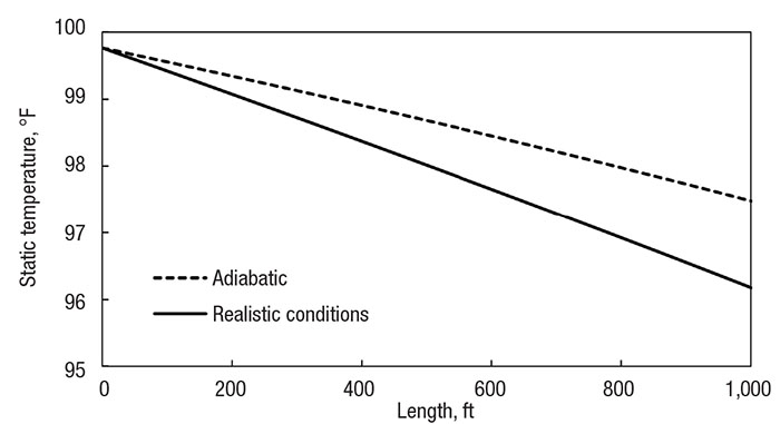
Figure 2. Comparing the adiabatic assumption (dotted line) with realistic heat transfer (solid line) of a 1,000 ft (300 m) pipe with a 3-in. (7.5 cm) diameter 1-in. (2.5 cm) thick insulation
Notice how the fluid experiences small, but noticeable, adiabatic cooling. Because the pipe is relatively short, and there is little pressure difference across the pipe, the velocity does not increase much, so the enthalpy change is slight. The important takeaway from this figure is to visualize how the adiabatic case matches with real conditions in a short, insulated pipe. The results are within 1.5°F (1°C) of each other.
The other common assumption in gas processes is isothermal flow. The prefix “iso” means “equal”, so isothermal flow means the temperature remains constant. Because gases tend to change temperature while flowing, heat transfer occurs between the system and its surroundings to keep the temperature from changing. So, this does not immediately simplify the energy balance as far as the adiabatic model; however, eliminating even one variable in compressible flow makes the problem much simpler. In this case, isothermal flow simplifies the equation of state for analysis at different points in the system. Heat transfer and flow analysis now revolve around knowing the temperature stays constant.
The isothermal assumption is applicable in systems where heat transfer is relatively rapid. For example, very long systems with little insulation experience fast heat transfer. When there is a temperature gradient between the system and outside surroundings, heat moves between the two such that the system fluid will approach the outside temperature. The faster the fluid temperature changes to match the surroundings, the longer the temperature remains constant after the fact.
A pattern of either exponential decay (outside temperature is lower) or logarithmic growth (outside temperature is higher) exists for the system fluid’s temperature. In either case, the beginning slope is always steeper than the end. The steeper the slope up front (faster heat transfer), the longer the fluid temperature profile is nearly flat. Therefore, engineers can approximate long pipes with rapid heat transfer as isothermal.
Isothermal flow can be applied whether heat is entering or leaving the system; the only criterion is that heat transfer is fast. No matter the direction of heat flow, velocity of the fluid increases with the dropping pressure, as in the adiabatic case. The major difference with isothermal flow, however, is that because temperature is constant, the corresponding volumetric flowrates and velocities are easier to predict if pressures are known. Only pressure and volume are variable in the equation of state for the gas, as opposed to adiabatic flow, which sees variable temperature as well.
Figure 3 presents the temperature profile of the methane-transfer system assuming isothermal flow at the ambient temperature of 60°F (16°C). The pipe includes no insulation and has been adjusted to a length of nearly 20 miles (32 km) and diameter of 6 in. (15 cm). Superimposed on this graph is the corresponding profile of the realistic system model, which uses correlations from literature to determine the real heat-transfer effects of the surroundings. Notice how the temperatures are the same for the latter 90% of the pipe.
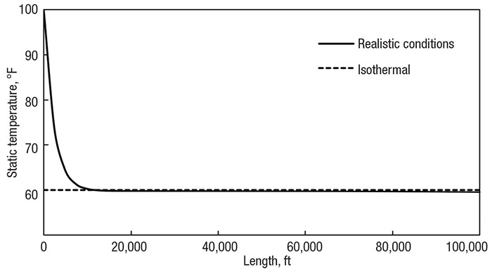
Figure 3. Comparing the isothermal assumption (dotted line) with realistic heat transfer (solid line) of a 100,000 ft (32,000 m) pipe with a 6 in. (15 cm) diameter and no insulation
While the temperatures are quite different at the beginning, the system quickly adjusts, so the flow behavior through the system is predictable. Also notice how real conditions cause the temperature to go slightly below ambient conditions. The flow naturally wants to drop temperature and relies on the surroundings to keep it constant. When the system and surrounding temperatures are so close, there is little heat transfer between them, and the enthalpy change scarcely dominates the heat rate in. However, for practical purposes, the temperature remains constant.
Changes to the real system
When comparing the above assumptions to realistic conditions, those real scenarios were tailored for the purpose of getting answers near their ideal counterparts. The pipes were made intentionally short or long, with little or much insulation to show when the assumptions can be properly applied. In the actual field, however, such tailoring is not possible. And it is unlikely to have a system that meets all the qualifications for the assumptions to be great approximations. Again, the engineer determines what is good enough.
If the system is, instead, a length of 2 miles (3 km) for analysis of both the adiabatic and isothermal cases, the simplifications come under scrutiny. The adiabatic case no longer has a short pipeline to help match reality. And the isothermal case no longer has such a long pipeline. The system is fixed to this new length, fixed to a 6 in. (15 cm) diameter, and fixed to insulation of 0.5 in. (1 cm). The real system, if already in existence, should guide the modeling and proposed simplifying assumptions. The assumptions should not come before the real system is understood. Given this system, is the adiabatic or isothermal assumption more appropriate? At first glance, an engineer could argue for either.
The pipe is longer and has less insulation than the previous adiabatic example. Heat transfer in the real conditions will now occur more rapidly. However, an engineer still may be tempted to assume adiabatic flow because the pipe is insulated, and there is not a relatively large temperature gradient between the system and surroundings. Also, depending on other systems in question, the pipeline may be short in comparison.
However, results show a large difference between the outlet temperatures. Figure 4 compares the temperature profiles of the new adiabatic and realistic models. (Notice, again, the small adiabatic cooling effect. The pressure is still not low enough to cause much difference in kinetic energy and enthalpy between the inlet and outlet.) Depending on the downstream process, this may or may not have a large impact of process reliability. Perhaps the methane enters a heat exchanger or combustion chamber, or perhaps it is branched off to deliver to residential neighborhoods. The performance and flow distribution will be affected, but sound engineering judgment is required to decide if the difference is important.
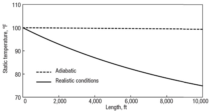
Figure 4. Comparing the adiabatic assumption (dotted line) with realistic heat transfer (solid line) of a 10,000 ft (3,000 m) pipe with a 6-in. (15 cm) diameter and 0.5-in. (1 cm) thick insulation
In the adiabatic case, the properties at the system outlet see the largest difference. As the system extends, the real heat transfer occurring has more influence, and the outlet conditions diverge further from adiabatic expectations. However, the system outlet is not the only area of concern in compressible flow. It tends to be the most obvious area to look because that is what directly leads to downstream processes, but the entire temperature profile needs to be analyzed.
For instance, the largest deviation isothermal flow has from real flow occurs at the inlet of the system. The system is now much shorter than the original example. It also contains some insulation, which slows the heat transfer, so the temperature profile is not as steep at the beginning. Figure 5 shows the different temperature profiles of the new real system and the isothermal case. Compare this to the original example in Figure 3. The real system now does not reach the surrounding temperature, but it could be considered close, depending on the engineer’s perspective. There is absolute deviation of 15°F (8°C), which is closer than the deviation of 25°F (14°C) from the adiabatic case.
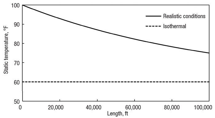
Figure 5. Comparing the isothermal assumption (dotted line) with realistic heat transfer (solid line) of a 10,000 ft (3,000 m) pipe with a 6-in. (15 cm) diameter and 0.5-in. (1 cm) thick insulation
Incorrect analysis is unlikely if the engineer is skeptical about that final difference. But if the engineer assumes the difference is no big deal, he or she needs to understand the upstream profile will differ even more so. While the system fluid still approaches the surrounding temperature, it does so much slower. Results at the outlet may falsely lead an engineer to believe an isothermal assumption is appropriate — the outlet properties can match somewhat well. And this may even be justified by the engineer claiming the pipe is long at 2 miles (3 km) and lightly insulated. However, the temperatures, flowrates and pressures are quite different along most of the pipe. This cannot be ignored.
Value of modeling software
These are mild examples of when the real case deviates from the ideal assumptions. The behavior will change depending on many factors, such as fluid, system scale, and process conditions. And the effects are more exaggerated when extreme conditions exist. Justifying assumptions as large as those discussed here can be the most difficult part of an engineer’s job. Knowing the amount of error that is reasonable for a model is no easy task. It is rarely obvious what assumptions are appropriate. That is the major problem when using qualifying terms like “long” and “rapid”.
The fact is a model can only be truly validated when comparing to field data. When measured data come back significantly different from the simplified model, explanation is required, but often dreaded, by the engineer. So, why do engineers have to make such simplifications in the first place? It is to untangle the math and get answers promptly, but we live in a day and age when computers do the heavy lifting.
Software allows an engineer to work through all the math (typically in a timelier manner) to obtain more accurate results. If the real conditions are different from what the ideal cases call for, then results will also differ. It depends on the engineering application whether that difference is a concern or not. For example, a controlled steam flow temperature to ensure condensation does not happen prematurely may be more important than controlling the temperature of air through pneumatic tools. However, with the complex coupling of many variables in compressible flow, being inaccurate in one variable means inaccuracy of many more. It is not so simple as choosing one property that can have large error. All properties need to come into consideration.
No system is perfectly insulated, and no pipeline is truly isothermal. When simplifications are made, error will result. The goal of the engineer should be to match mathematical models as close to reality as is reasonable and in as timely a manner as possible. The best way to accomplish this is to use modeling software that does not rely on such simplifications as incompressible solution methods or adiabatic or isothermal flow. Those may be useful for first-pass hand calculations but should not be relied upon for in-depth analysis. Compressible flow has many more complications than discussed here, such as sonic choking, so considering those affects only makes analysis harder. Do not sacrifice model quality for calculation ease. Better tools exist to help.
Reference
1. This model, and all output, was created using AFT Arrow software.
 Walt Prentice is a business applications engineer at Applied Flow Technology (AFT; 2955 Professional Pl, Colorado Springs, CO 80904; Phone: 719-686-1000; Fax: 719-686-1001; Email: walt.prentice@aft.com). He holds a B.S.Ch.E. degree, with a minor in economics, from the Colorado School of Mines.