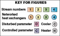
The ever important aim of energy efficiency in the chemical process industries (CPI) is brought closer to its target by the practice of energy recovery in heat exchanger networks (HENs). When heat exchangers are designed to work together to exchange heat between hot and cold streams, the required utilities are effectively reduced. The HEN designer usually applies the assumptions of fixed operating parameters at nominal conditions for given specifications of a process. But practically, a HEN should remain operable under variations in operating conditions without losing stream temperature targets and, at the same time, maintain economically optimal energy integration.
This article illustrates how to use sensitivity tables to design an optimum, flexible HEN for a multi-period process that is feasible for N periods of operations. The sensitivity tables approach is developed, automated and illustrated on an example problem.
The approach is applied through two steps. The first one is developing a strategy for the choice of the HEN’s base case, upon which sensitivity tables are generated. The second step is using sensitivity tables to reach target temperatures, and hence, target utilities of the alternative cases. In the end, we can have a HEN that realizes maximum energy savings under different operating conditions — in other words, a HEN with flexible and optimum properties.
Design of optimal, flexible HEN
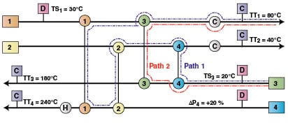
The sensitivity tables approach.The use of sensitivity tables replaces rigorous simulation to study the passive response of internal and target network temperatures to changes in supply temperatures, heat capacity flowrates and effective values of heat transfer coefficients for the heat exchangers. Moreover, combined actions can be considered using sensitivity tables where tradeoff between energy, capital cost and flexibility can be established. The new mode of operation can be considered as a deviation from the base case, so it represents the disturbances in supply and target temperatures, and even heat capacity flowrates. Disturbances may occur for short or long periods where, certain parameters have to be fixed. These parameters are called controlled parameters (C) and disturbed parameters (D). The period for which the disturbances equal zero is called the “base case”, such a case to be identified and presented on a grid diagram pointing out all the internal network temperatures before any analysis is performed.
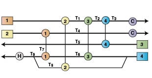
Downstream paths.A path is an unbroken connection between any two points in the grid diagram (Figure 1). Propagation of a disturbance at point D on Stream 3 along the downstream path, Path 2, would affect the controlled target temperature of Stream 1 (TT1). The propagation of the disturbance along the upstream path, Path1, would not influence TT1. For corrective actions and to maintain a required C (in this case, TT1), modifications of the heat exchangers by changing their effective UA will be considered as disturbances to counter balance the original disturbances. Consequently the exchanger having a downstream path into the controlled parameter is a candidate exchanger for contingency [23].
 |
|
 |
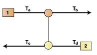 |
The sensitivity tables.The magnitude of the effect caused by D on C and the way to eliminate this effect are established by introducing the sensitivity tables approach [23]. The generation of sensitivity tables is based on the simple heat transfer equations of the heat exchanger. For a single heat exchanger shown in Figure 2, the heat balance equations are:
Q = CP H (T a – T b) (1)
= CP C (T d – T c) (2)
= UA (Δ T LM) (3)
(4)
Where Q is the exchanger heat load, CP H, CP C are the hot and cold heat capacity flowrates for the hot and cold streams respectively, U is the overall heat transfer coefficient, A is the heat transfer area and Δ T LMis the log mean temperature difference.
The following new variables (R and B) were introduced:
R = CPC / CPH (5)
B = Exp [ UA / CPC(R –1)] (6)
Using Equations (1–6) Kotjabasakis and Linnhoff [ 23] generated the following two equations:
(1– RB) T b + (B –1) RT c + (R –1) T a = 0.0 (7)
R (1– RB) T d + (B –1) RT a + (R –1) BRT c = 0.0 (8)
Equations (7) and (8) are linear with respect to temperature and nonlinear with respect to both heat capacity flowrates and UA s. For the same heat exchanger in Figure 2, knowing two of the four temperatures (Ta, T b, T c, T d) and knowing UA, CP H and CP C, the other two temperatures can be determined by solving Equations (7) and (8). This way of formulation is effective for each exchanger in any feasible network. Once the overall system of equations is solved for each exchanger in the base case, new network temperatures can be determined when changes occur in supply temperatures, heat capacity flowrates and effective UA s.
Constructing sensitivity tables. Three types of sensitivity tables can be constructed, where they simply correlate the response of the network temperatures to changes of input stream temperatures (T S), heat capacity flowrates (CP) and the UA of the networked exchangers. The information needed are the base case stream data and the network structure. The different types of sensitivity tables are as follows:
1. T(TS) sensitivity tables: These tables correlate the response of the network temperatures to unit variation of input stream temperatures. One table is enough to describe the responses to changes in all stream supply temperatures.
2. T(CP) sensitivity tables: These tables correlate the response of the network temperatures according to changes in heat capacity flowrate for a specific stream. Because Equations (7) and (8) are non linear with respect to CP, the CP sensitivity tables are constructed for different levels of CP variation in a specific stream. Interpolation between these values is possible.
3. T(UA) sensitivity tables: These tables need to be constructed for each individual heat exchanger in the network. These tables correlate the response of the network temperatures to changes of the effective exchanger (in terms of UA). Because Equations (7) and (8) are non linear with respect to UA, the temperatures responses are evaluated at different values of UA percent of every effective heat exchanger of the base case network.
Using sensitivity tables. Once sensitivity tables have been constructed for the base case, the variation of any of the network temperatures can be calculated by simple summation of the variations resulting from individual disturbances (supply stream temperatures and stream heat-capacity flowrates). Sensitivity tables for UA can then be utilized for contingency-candidate exchangers in order to quantify the necessary change in exchangers’ UA values that rectify the disturbances [23]. We assume that for each period, adjusting stream temperatures at the inlet of utilities can be used to nearly match target utility requirements determined via the pinch design method (PDM), which was developed by Linnhoff and his colleagues [24].
Conclusion
The sensitivity tables approach can be used to design optimal flexible HEN for multiperiods process. The tables are constructed by detecting the variations of the base case temperatures due to disturbances in streams supply temperatures, heat capacity flowrates and heat transfer coefficients (through UAs). Then, the sensitivity tables are used to adjust the streams’ target temperatures to achieve target utility requirements as close as possible to PDM results for each period by adjusting candidate downstream heat exchangers’ UA contingencies. Using PDM design at each period can evolve a flexible HEN design much easier than using sensitivity tables. However, sensitivity tables are more suitable to retrofit HEN to render it flexible for limited variations in process parameters.
Illustration of the approach
We have applied the sensitivity tables approach on a literature problem (Example 1 in Ref. 8, a process that has three modes of operation (defined as Periods 1 through 3). The conditions of the process changes periodically over the year. Each period differs from other periods in supply, target temperatures and in heat capacity flowrates. The problem data are given in Table 1.
| Table 1. Stream Data for the Example Problem | ||||
| CP, kW / ºC | TTi, ºC | TSi, ºC | Stream No. | Case No. |
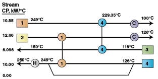
| 10.55 | 100 | 249 | 1 | Base Case Period 1 |
| 12.66 | 128 | 259 | 2 | |
| 9.144 | 170 | 96 | 3 | |
| 15.00 | 270 | 106 | 4 | |
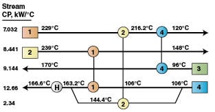
| 7.032 | 120 | 229 | 1 | Period 2 |
| 8.44 | 148 | 239 | 2 | |
| 9.144 | 170 | 96 | 3 | |
| 15.00 | 270 | 106 | 4 | |
| 10.55 | 100 | 249 | 1 | Period 3 |
| 12.66 | 128 | 259 | 2 | |
| 6.096 | 150 | 116 | 3 | |
| 10.00 | 250 | 126 | 4 | |
Construction of sensitivity tables for the problem. In order to apply the sensitivity tables approach, we must define the base case for the HEN design upon which the sensitivity tables will be generated.
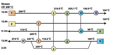
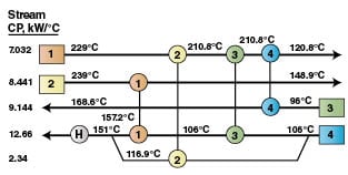
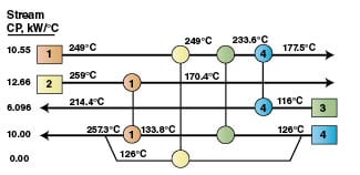
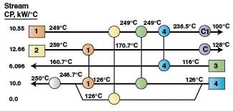
Utility targeting and selection of the HEN’s base case. The PDM has been applied on the three periods of the process to locate the pinch points, minimum utilities consumption and minimum number of units and to establish matches for each period (Figures 3, 4 and 5). Table 2 displays minimum utilities consumption and pinch location for each period of the problem. The base case is chosen as the HEN containing the largest number of units (Period 1). By inspection of the three periods’ HEN, it can be concluded that almost all equipment required in Periods 2 and 3 can all be covered by matches in Period 1. Only the cooler of Stream 2 in Period 3 will be added to the HEN of Period 1. This will be the base case, and the temperature diagram of the problem is shown in Figure 6.
 |
 |
 |
 |
| Table 2. Minimum Utilities Requirements and Pinch Points for the Example Problem using the PDM Method | |||
| Period No. | Pinch point, °C | Minimum hot utility, kW | Minimum cold utility, kW |
| 1 | 249 – 239 | 338.4 | 432.15 |
| 2 | 1,602.13 | 0.0 | |
| 3 | 249 – 259 | 10.00 | 1,793.15 |
Generation of the sensitivity tables.Now, we have a HEN base-case design with four heat exchangers as shown in Figure 6. The internal network temperatures (T i generically, or T 1 through T 9 in this case), heat exchanged and UA for each heat exchanger are calculated. Then, the variables R and B for each heat exchanger are determined using Equations (5) and (6). Then, Equations (7) and (8) are constructed for each heat exchanger (see Figure 2). Eight equations, two for each exchanger, were solved for the internal temperatures shown in Figure 6. A value for T 9 is obtained from T 7 and T 8.
We considered that all start temperatures are disturbed [D] and all target temperatures are fixed, controlled [C].
Keeping other conditions at the base case values, the equations have been solved for the following cases:
1. A positive unit change in the disturbed temperature, one at a time.
2. Variable percent change in CP from the base case for each stream.
3. Variable percent change in UA from the base case for each exchanger.
The sensitivity tables for the problem are listed in Tables 3–8. They represent the response of network temperatures resulting from the variation listed above.
|
Table 3. Example T(TS) Sensitivity Table (for each 1°C change in Ts) |
||||
| ∆Ti, ºC | Stream 1 | Stream 2 | Stream 3 | Stream 4 |
| ∆T1 | .794 | 0.0 | 0.0 | 0.0 |
| ∆T2 | .693 | 0.0 | 0.0 | .127 |
| ∆T3 | .283 | 0.0 | .634 | .098 |
| ∆T4 | .077 | .081 | 0.0 | .841 |
| ∆T5 | .469 | 0.0 | .341 | .106 |
| ∆T6 | .094 | 0.0 | 0.0 | .695 |
| ∆T7 | .033 | .38 | 0.0 | .043 |
| ∆T8 | .930 | 0.0 | 0.0 | 0.0 |
| Table 4. The T(CP) Sensitivity Table for the Example Problem | |||||
| ∆Ti, ºC | ∆CP1 –33.34 % | ∆CP2 –33.34 % | ∆CP3 –33.34 % | ∆CP4 –21.01 % | ∆CP5 –100 % |
| ∆T1 | –13.959 | 0.0 | 0.0 | 0.0 | 29.499 |
| ∆T2 | –17.912 | 0.0 | 0.0 | .19951 | 25.756 |
| ∆T3 | –23.384 | 0.0 | 11.134 | .128 | 10.656 |
| ∆T4 | –1.667 | –9.932 | 0.0 | 22.702 | 2.908 |
| ∆T5 | –20.420 | 0.019 | 17.840 | .1545 | 17.490 |
| ∆T6 | –2.0051 | 0.199 | 0.0 | 2.782 | 2.920 |
| ∆T7 | –.6772 | –37.586 | 0.0 | 8.537 | –.328 |
| ∆T8 | –2.400 | 0.0 | 0.0 | 0.0 | 10 |
| Table 5. T (UA) Sensitivity Table for Exchanger No.1 of the Example Problem | |||||||||||
| % Change in UA from the base case | |||||||||||
| ∆Ti, ºC | + 100 % | +80 % | +60 % | +40 % | +20 % | 0 % | –20% | –40 % | –60 % | –80 % | –100 % |
| ∆T1 | 0.0 | 0.0 | 0.0 | 0.0 | 0.0 | 0.0 | 0.0 | 0.0 | 0.0 | 0.0 | 0.0 |
| ∆T2 | 0.0 | 0.0 | 0.0 | 0.0 | 0.0 | 0.0 | 0.0 | 0.0 | 0.0 | 0.0 | 0.0 |
| ∆T3 | 0.0 | 0.0 | 0.0 | 0.0 | 0.0 | 0.0 | 0.0 | 0.0 | 0.0 | 0.0 | 0.0 |
| ∆T4 | –4.808 | –4.25 | –3.57 | –2.7 | –1.56 | 0.0 | 2.29 | 5.93 | 12.61 | 28.97 | 131 |
| ∆T5 | 0.0 | 0.0 | 0.0 | 0.0 | 0.0 | 0.0 | 0.0 | 0.0 | 0.0 | 0.0 | 0.0 |
| ∆T6 | 0.0 | 0.0 | 0.0 | 0.0 | 0.0 | 0.0 | 0.0 | 0.0 | 0.0 | 0.0 | 0.0 |
| ∆T7 | 4.27 | 3.72 | 3.03 | 2.16 | 1.019 | 0.0 | –2.83 | –6.47 | –13.15 | –29.51 | –131.6 |
| ∆T8 | 0.0 | 0.0 | 0.0 | 0.0 | 0.0 | 0.0 | 0.0 | 0.0 | 0.0 | 0.0 | 0.0 |
| ∆T9 | 4.07 | 3.601 | 3.023 | 2.288 | 1.324 | 0.0 | –1.93 | –4.993 | –10.64 | –24.44 | –110.6 |
| Table 6. T (UA) Sensitivity Table for Exchanger No.2 of the Example Problem | |||||||||||
| % Change in UA from the base case | |||||||||||
| ∆Ti, ºC | + 100 % | +80 % | +60 % | +40 % | +20 % | 0 % | –20% | –40 % | –60 % | –80 % | –100 % |
| ∆T1 | –2.026 | –1.905 | –1.709 | –1.388 | –0.863 | 0.0 | 1.433 | 3.842 | 7.979 | 15.366 | 29.5 |
| ∆T2 | –1.769 | –1.663 | –1.492 | –1.212 | –0.754 | 0.0 | 1.252 | 3.354 | 6.967 | 13.416 | 25.76 |
| ∆T3 | –0.683 | –0.64 | –0.569 | –0.454 | –0.265 | 0.0 | .561 | 1.427 | 2.916 | 5.572 | 10.66 |
| ∆T4 | –0.189 | –0.177 | –0.157 | –0.126 | –0.07 | 0.0 | .151 | .388 | .794 | 1.52 | 2.91 |
| ∆T5 | –1.181 | –1.11 | –0.993 | –0.8033 | –0.492 | 0.0 | .868 | 2.295 | 4.746 | 9.12 | 17.49 |
| ∆T6 | –0.413 | –0.401 | –0.38 | –0.346 | –0.290 | 0.0 | –0.048 | .2071 | .645 | 1.426 | 2.92 |
| ∆T7 | –0.564 | –0.563 | –0.562 | –0.5596 | –0.556 | 0.0 | –0.538 | –0.520 | –0.489 | –0.434 | –0.328 |
| ∆T8 | 9.135 | 8.592 | 7.71 | 6.262 | 3.895 | 0.0 | –6.460 | –17.32 | –35.97 | –69.27 | –133 |
| Table 7. T (UA) Sensitivity Table for Exchanger No.3 of the Example Problem | |||||||||||
| % Change in UA from the base case | |||||||||||
| ∆Ti, ºC | + 100 % | +80 % | +60 % | +40 % | +20 % | 0 % | –20% | –40 % | –60 % | –80 % | –100 % |
| ∆T1 | 0.0 | 0.0 | 0.0 | 0.0 | 0.0 | 0.0 | 0.0 | 0.0 | 0.0 | 0.0 | 0.0 |
| ∆T2 | –11.4 | –9.31 | –7.14 | –4.86 | –2.49 | 0.0 | 2.61 | 5.34 | 8.21 | 11.22 | 14.4 |
| ∆T3 | –4.65 | –3.79 | –2.89 | –1.96 | –0.98 | 0.0 | 1.12 | 2.24 | 3.43 | 4.67 | 5.98 |
| ∆T4 | 8.83 | 7.22 | 5.54 | 3.78 | 1.94 | 0.0 | –2.01 | –4.12 | –6.34 | –8.67 | –11.14 |
| ∆T5 | –7.71 | –6.3 | –4.82 | –3.28 | –1.67 | 0.0 | 1.79 | 3.64 | 5.59 | 7.63 | 9.79 |
| ∆T6 | 9.3 | 7.56 | 5.75 | 3.85 | 1.87 | 0.0 | –2.37 | –4.65 | –7.04 | –9.55 | –12.2 |
| ∆T7 | 0.12 | 0.001 | –0.13 | –0.26 | –0.40 | 0.0 | –0.70 | –0.86 | –1.03 | –1.21 | –1.4 |
| ∆T8 | 0.0 | 0.0 | 0.0 | 0.0 | 0.0 | 0.0 | 0.0 | 0.0 | 0.0 | 0.0 | 0.0 |
| Table 8. T (UA) Sensitivity Table for Exchanger No. 4 of the Example Problem | |||||||||||
| % Change in UA from the base case | |||||||||||
| ∆Ti, ºC | + 100 % | +80 % | +60 % | +40 % | +20 % | 0 % | –20% | –40 % | –60 % | –80 % | –100 % |
| ∆T1 | 0.0 | 0.0 | 0.0 | 0.0 | 0.0 | 0.0 | 0.0 | 0.0 | 0.0 | 0.0 | 0.0 |
| ∆T2 | 0.0 | 0.0 | 0.0 | 0.0 | 0.0 | 0.0 | 0.0 | 0.0 | 0.0 | 0.0 | 0.0 |
| ∆T3 | –14.1 | –12.24 | –10.03 | –7.36 | –4.08 | 0.0 | 5.39 | 12.57 | 22.71 | 38.1 | 64.2 |
| ∆T4 | 0.0 | 0.0 | 0.0 | 0.0 | 0.0 | 0.0 | 0.0 | 0.0 | 0.0 | 0.0 | 0.0 |
| ∆T5 | 16.3 | 14.19 | 11.64 | 8.57 | 4.78 | 0.0 | –6.15 | –14.43 | –26.13 | –43.9 | –74 |
| ∆T6 | 0.0 | 0.0 | 0.0 | 0.0 | 0.0 | 0.0 | 0.0 | 0.0 | 0.0 | 0.0 | 0.0 |
| ∆T7 | 0.0 | 0.0 | 0.0 | 0.0 | 0.0 | 0.0 | 0.0 | 0.0 | 0.0 | 0.0 | 0.0 |
| ∆T8 | 0.0 | 0.0 | 0.0 | 0.0 | 0.0 | 0.0 | 0.0 | 0.0 | 0.0 | 0.0 | 0.0 |
Synthesizing an optimal flexible HEN for Period 2.The disturbances in Period 2 are due to variations in T S 1, T S 2, CP 1 and CP 2. The disturbance in the different network temperatures is calculated as follows:
∆T i = ∆T i < T S 1> + ∆T i < T S 2>
+ ∆T i < CP 1> + ∆T i < CP 2> (9)
Where
∆T i < T S 1> is the change in T i as a consequence of D in T S 1.
∆T i < T S 2> is the change in T i as a consequence of D in T S 2.
∆T i < CP 1> is the change in T i as a consequence of D in CP 1.
∆T i < CP 2> is the change in T i as a consequence of D in CP 2
∆T i is the change in T i due to the combined disturbances.
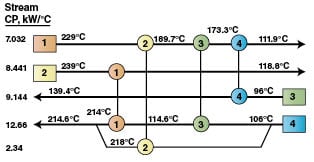
By using the sensitivity tables (Tables 3, 4) and applying Equation (9) we can deduce the internal temperatures of the network as a result of combined disturbances for Period 2 (Figure 7).
Example calculation for ∆T 1: If T S 1 in Period 2 is 20°C lower than in the base case, and the T S sensitivity table (Table 3) shows that ∆T 1 is 0.794 for each 1°C temperature disturbance in T S 1, then:
∆T 1= (0.794)(–20) + (0.0)(–20) + (–13.95) + (0.0) = –29.83ËšC
By comparing Figures 4 and 7, we find variations in target temperatures due to the combined effect of variations in target temperatures from the base case and Period 2 (Table 1) and the disturbances in the streams’ inlet temperatures and heat capacity flowrates. The target temperatures in Figure 7 need to be adjusted to those shown in Figure 4 by an increase or decrease in each heat exchanger’s UA, but at the same time utilities need to be kept as close as possible to the target minimum values predicted by PDM. By using the downstream paths, we can detect the candidate heat exchangers for adjusting each UA. Using the UA sensitivity tables (Tables 5–8) and after several trials, the contingency for each exchanger’s UA (< UA j> for j =1 to 4) was found as follows: < UA 1> = –87%, < UA 2> = –90%, < UA 3> = –100%, < UA 4> = +27%
The final network with corrected internal and target temperatures is generated using the adjusted heat exchangers’ UA through Equations (10) and (11), where the final disturbance in network temperatures is the summation of individual disturbances due to contingencies in the exchangers’ UA s:
(10)
Where ∆ T i < UA > j is the disturbance in network temperature resulting from using UA contingency in exchanger j. In this case, the number of exchangers ( n) is 4.
T i ( new ) = T i ( disturbed ) + ∆ T i (11)
Where:
∆ T i is the final disturbance in internal network temperature resulting from using UA contingences.
T i ( new ) is the new (or final) calculated internal network temperature.
T i ( disturbed ) is the old internal temperatures of the network as a result of the change in operating conditions.
The final network for Period 2 that is both flexible and optimized is shown in Figure 8. It can be seen that streams’ temperatures before utility use are very close to those of Figure 4.
 |
 |
 |
 |
Synthesizing an optimal, flexible HEN for Period 3.The steps applied to reach to a flexible, optimum HEN design for Period 2, can be applied again for Period 3. Sensitivity tables 3–8 are used to detect and correct disturbances of network, due to changes in supply temperatures, capacity flowrates and target temperatures. In this case since Stream 5, a branch of Stream 4, has been canceled ( CP 5 = 0.0), then automatically Exchanger 2 is deleted. Only the disturbance resulting from Stream 5 cancellation is taken into consideration when calculating the overall disturbances’ effect. HEN for Period 3 with disturbed temperatures is shown in Figure 9. The T ( UA) tables are used to establish the exchangers UA contingencies to adjust the target temperatures of network. The best achieved results are as follows: = –56 %, = –100 %, = –100%, = –93 %.
The final Network for Period 3 is shown in Figure 10. In this case we were not able to achieve the required target temperatures using sensitivity tables; a deviation of 2.3–10°C from PDM results was noticed (Figure 5).
Comparison with PDM Design
It is interesting to find out whether PDM design can offer any insight to the flexibility problem. Indeed it does, as we mentioned before the matches for the three periods of operation are more or less identical, with one or more exchangers to be bypassed and the others to be adjusted for their UA s. Table 9 displays a comparison between UA contingencies as calculated from PDM and sensitivity tables for Periods 2 and 3 respectively. It is clear that there is fair agreement between the contingencies’ values calculated by both methods.
| Table 9. Comparison of UA Contingences Between Sensitivity Table and PDM for Period 2 and Period 3 | ||||
| UAi | Period 2 | Period 3 | ||
| Sensitivity table | PDM | Sensitivity table | PDM | |
| UA1 | –87% | – 92 % | –61 % | –63 % |
| UA2 | –90 % | –87 % | –100 % | –100% |
| UA3 | –100 % | –100 % | –100% | –100 % |
| UA4 | +27 % | + 17 % | –92 % | –88% |
Edited by Rebekkah Marshall
References
1. Furman, K. C., and Sahinidis, N. V., A Critical Review and Annotated Bibliography for Heat Exchanger Network Synthesis in the 20th Century, Ind. and Eng. Chem. Res., 41(10): 2335-2370, 2002.
2. Gundersen T., and Naess, L., The Synthesis of Cost Optimal Heat Exchanger Networks. Comp. and Chem. Eng., 12(6):503–530, 1988.
3. Ježowski, J., Heat Exchanger Network Grassroot and Retrofit Design. The Review of the State-of the-Art: Part I. Heat Exchanger Network Targeting and Insight Based Methods of Synthesis. Hungarian J. of Ind. Chem., 22:279–294, 1994.
4. Ježowski J., Heat Exchanger Network Grassroot and Retrofit Design. The Review of the State-of the-Art: Part II. Heat Exchanger Network Synthesis by Mathematical Methods an Approaches for Retrofit Design. Hungarian J. of Ind. Chem., 22:295–308, 1994.
5. Marselle, D. F., Morari, M. and Rudd, D.F., Design of Resilient Processing Plants–II. Design and Control of Energy Management Systems. Chem. Eng. Sci., 37(2):259–270, 1982.
6. Swaney, R.E., and Grossmann, I.E., An index for operational flexibility in chemical process design I:
Formulation and theory, AIChE J., 31: 621, 1985.
7. Floudas, C.A., and Grossmann, I.E., Automatic Generation of Multiperiod Heat Exchanger Network Configurations. Comp. and Chem. Eng., 11(2), pp. 123–142, 1987.
8. Floudas, C.A. and Grossmann, I.E., Synthesis of Flexible Heat Exchanger Networks for Multiperiod Operation. Comp. and Chem. Eng., 10(2), pp. 153–168, 1986.
9. Floudas, C.A., and Grossmann, I.E., Synthesis of Flexible Heat Exchanger Networks with Uncertain Flowrates and Temperatures. Comp. and Chem. Eng., 11(4), pp. 319–336, 1987.
10. Floudas, C.A., Ciric, A.R. and Grossmann, I.E., Automatic Synthesis of Optimum Heat Exchanger Network Configurations. AIChE J., 32(2), pp. 276–290, 1986.
11. Grossmann, I.E. and Floudas, C.A., Active Constraint Strategy for Flexibility Analysis in Chemical Processes. Comp. and Chem. Eng., 11(6), pp. 675–693, 1987.
12. Verheyen and Zhang, Design of Flexible Heat Exchanger Network for Multi-Period Operation, Chem. Eng. Sci., 61, pp. 7730–7753, 2006.
13. Yee, T. F., Grossmann, I.E., and Kravanja, Z., Simultaneous Optimization Models for Heat Integration–I. Area and Energy Targeting and Modeling of Multi-Stream Exchangers. Comp. and Chem. Eng., 14(10), p. 1151–1164, 1990.
14. Yee, T. F., and Grossmann, I.E.,, Simultaneous Optimization Models for Heat Integration–II. Heat Exchanger Network Synthesis. Comp. and Chem. Eng., 14(10):1165–1184, 1990.
15. Aaltola J., Simultaneous synthesis of flexible heat exchanger network. App. Therm. Eng., 22(8), pp. 907–918, 2002.
16. Aguilera, N., and Nasini, G., Flexibility Test for Heat Exchanger Networks with Uncertain Flowrates. Comp. and Chem. Eng., 19(9):1007–1017, 1995.
17. Aguilera, N., and Nasini, G., Flexibility Test for Heat Exchanger Networks with Non-overlapping Inlet Temperature Variations, Comp. and Chem. Eng., 20(10):1227–1240, 1996.
18. Tantimuratha L., Asteris, G., Antonopoulos, D. K. and Kokossis, A. C., A conceptual programming approach for the design of flexible HENs. Comp. and Chem. Eng., 25 (4–6): 887–892, 2001.
19. Briones V. and Kokossis, A.C., Hypertargets: A Conceptual Programming Approach for the Optimization of Industrial Heat Exchanger Networks–I. Grassroots Design and Network Complexity. Chem. Eng. Sci., 54:519–539, 1999.
20. Briones V. and Kokossis, A. C. Hypertargets: A Conceptual Programming Approach for the Optimization of Industrial Heat Exchanger Networks–II. Retrofit Design. Chem. Eng. Sci., 54:541–561, 1999.
21. Briones V. and Kokossis, A. C., Hypertargets: A Conceptual Programming Approach for the Optimization of Industrial Heat Exchanger Networks–Part III. Industrial Applications. Chem. Eng. Sci., 54:685–706, 1999.
22. Konukman, A. E., Camurdan, M. C. and Akman, U., Simultaneous Flexibility Targeting And Synthesis Of Minimum-Utility Heat-Exchanger Networks With Superstructure-Based MILP, Chem. Eng. and Proc., 41(6): 501–518, 2002.
23. Kotjabasakis, E., and Linnhoff, B., Sensitivity Tables for the Design of Flexible Processes (1) – How Much Contingency in Heat Exchanger Networks Is Cost Effective. Chem. Eng. Res. Des., 64(3):197–211, 1986.
24. Linnhoff, B., Townsend, D.W., and Boland, D. “User Guide on Process Integration for the Efficient of Energy”, The Institution of Chemical Engineers. Warwick Printing Company Ltd., Great Britain, 1982.
Authors

Seham Ali El-Temtamy is a professor of chemical engineering at the Egyptian Petroleum R