The Joukowsky equation is often relied upon to determine the maximum possible fluid pressure inside a pipe, but there are certain scenarios where this equation does not return the expected conservative result for overpressurization
We engineers love our formulas. Especially when we know they can quickly give us a conservative, worst-case answer.
As a young engineer in the aerospace and power industries, I participated in multiple meetings and read several reports that used the Joukowsky equation to determine a maximum possible fluid pressure inside a pipe. Since everyone “knew” that the Joukowsky equation predicted the maximum possible pressure, this was a quick and reasonable thing to do. Unbeknownst to my managers, colleagues and myself at the time, this was a potentially dangerous thing to do. Because while the Joukowsky equation often returns a conservative result, it cannot be relied upon to do so in every situation.
This article summarizes the important points of a recent journal article [1] that discusses three different situations for which the Joukowsky equation does not give a worst-case, conservative answer.
The Joukowsky equation
The Joukowsky equation [2] relates the instant change in piezometric (hydraulic) head, H, to an instant change in velocity, V, often conceptualized as an instantaneous valve closure. The Joukowsky equation is sometimes referred to by other names, such as the “Basic Waterhammer Equation,” the “Instantaneous Waterhammer Equation” or the “Maximum Theoretical Waterhammer Equation.” The relationship is shown in Equation (1):
∆HJ = – a∆V⁄g (1)
where a is the wavespeed (also known as the celerity) and g is the acceleration due to body forces (32.2 ft/s2 or 9.8 m/s2 for stationary systems at the earth’s surface) due to gravity. The wavespeed is related to the speed of sound in the liquid, but also includes pipe structural interaction. Note that the negative sign in Equation (1) means that a reduction in velocity leads to an increase in piezometric head. Equation (1) is more typically found in civil engineering applications, which frequently use piezometric head and hydraulic gradeline concepts.
The relationship between the change in piezometric head and pressure, P, is given by Equation (2):
∆P = ρg∆H (2)
where ρ is the liquid density.
Combining Equations (1) and (2) results in a form of the Joukowsky equation that is more frequently used by chemical and mechanical engineers (Equation (3)).
∆PJ = –ρa∆V (3)
Equations (1) and (3) are essentially equivalent ways of presenting the Joukowsky Equation, and will be used interchangeably in this article. Note that one limitation of Equation (1) is that when the system experiences zero gravity, Equation (1) would have a divide-by-zero problem. In such cases, Equation (3) retains validity and is thus preferred. During my time working in the aerospace industry, I frequently worked on zero- g systems, as well as those with much higher and lower body forces than 1 g (1 standard earth gravitational acceleration). See Ref. 1 for more on this.
The Joukowsky equation traces its history back to the 19th century. In fact, Joukowsky is the lucky author whose name is most often associated with Equations (1) and (3). However, a thorough review of the early literature shows that others derived this equation prior to Joukowsky — for applications in blood flow [3].
Limiting assumptions
Before discussing the cases where the Joukowsky equation does not result in a conservative answer, it should be realized that the equation has numerous limiting assumptions. From Ref. 1:
“ In principle, Equation 1 only claims validity the moment after the velocity decrease (e.g., valve closure). However, practicing engineers often apply it as if it retains validity both immediately after the velocity decrease/valve closure, as well as at all times thereafter, assuming that no other independent transients occur. Since Equation 1 is often applied in this manner, the limitations of this equation are discussed with respect to its validity after the initial transient occurs. These limitations are as follows:”
• Straight, constant-diameter piping of uniform material, wall thickness and structural restraints
• Uniform pipe friction
• Minimal friction pressure drop in piping (explained in a later section)
• Minimal fluid-structure interaction with the piping and supports
• No cavitation or gas release
• No trapped, or entrained, gases in the piping (that is, it is initially 100% full of liquid)
• No external heat transfer that can change any of the piping and fluid physical properties or cause phase changes
• Constant liquid density and constant bulk modulus
• One-dimensional fluid flow
• Linearly elastic piping material
Example 1: Instant valve closure. Let’s take a look at a simple example from Ref. 1. Consider a pipe of diameter ( D) 0.5 m (1.64 ft) conveying oil with a specific gravity of 0.9 (the density, ρ, is 900 kg/m3, or 56.2 lbm/ft3). The volumetric flowrate, Q, is 0.4 m3/s (14.1 ft3/s) and the wavespeed, a (the propagation speed of the fluid transient), is 1,291 m/s (4,236 ft/s).
The pipe cross-sectional area, A, is given by Equation (4):
A = πD2/4 = 0.196 m2 (or 2.11 ft2) (4)
Hence, the velocity change if a valve is closed instantly can be calculated with Equation (5).
ΔV = ΔQ/A = –2.04 m/s (or –6.68 ft/s) (5)
Therefore, from Equation (1):
ΔHJ = – aΔV/g = –(1,291 m/s)( –2.04 m/s) / (9.81 m/s2) = 268 m (or 880 ft) (6)
And using Equation (3):
ΔPJ = –ρaΔV = –(900 kg/m3)(1,291 m/s)( –2.04 m/s) = 2,367 kPa (or 343 psi) (7)
Note that the value given by Equation (7) is the pressure increase due to waterhammer after an instant valve closure. To find the maximum pressure, the Equation (7) pressure increase must be added to the fluid’s pre-existing, steady-state pressure.
Cases where the equation does not give a conservative result
Three situations where Equation (3) may not be conservative are: transient cavitation and liquid column separation; line pack; and piping system reflections (networks, components, area changes and surge-suppression devices).
These three cases will be explored in three examples discussed below.
As chemical engineers are keenly aware, when liquid pressure drops to the local vapor pressure, the liquid will flash and vapor will be generated. This is called transient cavitation. It is transient because in a waterhammer situation, a reflecting transient pressure wave will typically and quickly repressurize the pipe and collapse the vapor. It is usually not a sustained, two-phase flow situation, but a temporary two-phase situation that quickly returns to single-phase in most cases.
If enough vapor is generated and flow conditions are right, the entire cross section of fluid can vaporize and the continuous column of liquid will have a vapor gap. This is true liquid column separation. In common use, transient cavitation and liquid column separation are synonymous terms.
It turns out that predicting the waterhammer pressure transients during and after transient cavitation has occurred is very difficult. The best available models are not very accurate, because the phenomenon is quite complex. As a result, waterhammer engineers treat predictions from simulation software in cases where transient cavitation occurs with great caution [4].
Moreover, it has been shown experimentally that when transient vapor pockets collapse, the resulting pressure spike can exceed the values returned by using Equation (3). Example 2 discusses this.
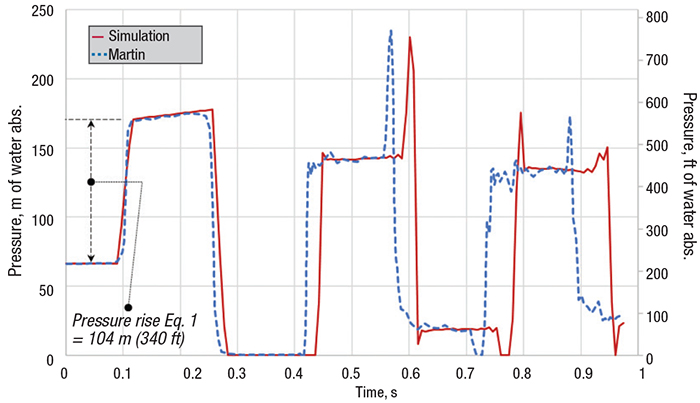
FIGURE 1. The graph shown here, from Example 2, illustrates the experimental and numerical predictions of pressures during transient cavitation, compared to the maximum predicted pressure from the Joukowsky equation (from Ref. 1)
Example 2: Transient cavitation and vapor collapse. Figure 1 shows the experimental results [5] and the commercial software simulation results [6] for a 102-m (335 ft) coiled copper tube experiencing waterhammer. Equation (1) predicts a maximum pressure rise of 104 m (340 ft), resulting in a peak pressure (when added to the steady-state pressure) of 171 m (560 ft) near 0.1 s. Thus, the initial pressure rise agrees with Equation (1). However, the reflecting wave leads to a pressure decrease, and transient cavitation begins at this location at about 0.3 s. It lasts until just after 0.4 s. This is the point at which the system repressurizes and collapses the vapor cavity. Both the experiment and the simulation show a peak pressure that exceeds the result from Equation (1) at about 0.6 s. This peak is about 235 m (770 ft). Ref. 1 offers guidance on how to quickly check for the possibility of transient cavitation in your system.
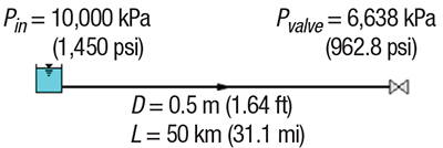
FIGURE 2. The diagram shows the system description for the horizontal pipe in Example 3
Example 3: Line pack: recovery of frictional pressure drop. The term “line pack” is commonly used, but is not very descriptive of the process. So before trying to describe what the term is, consider a simple conceptual example. First, just think about a steady-state situation. Figure 2 shows a 50-km horizontal pipeline with conditions taken from Example 1. Additional details for the steady-state input data for Example 3 are shown here:
L = 50 km (31.1 mi)
D = 0.5 m (1.64 ft)
f = 0.018
Q = 0.4 m3/s (14.1 ft 3 /s), 1,440 m3/h (6,340 gal/min)
V = 2.04 m/s (6.68 ft/s)
Pin = 10,000 kPa (1,450 psi), fixed
Pvalve = 6,638 kPa (962.8 psi), upstream initial pressure
ΔPpipe = 3,362 kPa (487.6 psi), initial pipe pressure drop
ρ = 900 kg/m3 (56.2 lbm/ft3)
The steady-state pressure drop is a simple calculation once the friction factor is determined (the Darcy-Weisbach f = 0.018). The pressure drop is thus 3,362 kPa (488 psid).
The question we ask here is: What is the pressure at the valve after it has closed, the flow has stopped, and all transients have died out? The answer is trivial. Since the entire pipe is horizontal, the pipe will have a pressure everywhere along its length that is the same as the inlet pressure of 10,000 kPa (1,450 psia).
Notice what happened here. The pressure at the valve increased. By how much? It increased by 3,362 kPa (488 psi). In fact, it increased by the same amount as the frictional pressure drop while it was flowing. This pressure increase has nothing to do with waterhammer. It is merely the increase in pressure when frictional pressure loss is no longer occurring. We will call this pressure increase the friction recovery pressure, ΔPfr. In the present example, ΔPfr = 3,362 kPa (or 488 psi).
During a pipeline transient, the frictional behavior interacts with the acoustic nature of the waterhammer wave such that a passing wave does not bring the fluid to a complete rest, even after a valve is closed. Ref. 7 contains an excellent summary of line pack:
“In pipeline transients, frictional resistance to flow generates line packing, which is a sustained pressure increase in the pipeline behind the waterhammer wave front after the closure of a discharge valve. This phenomenon is of interest to cross-country oil pipelines and long water transmission mains because the sustained pressure increase can be very significant relative to the initial sudden pressure increase by waterhammer and can result in unacceptable overpressures.”
Ref. 7 offers a powerful new method to estimate the combined pressure rise due to line pack and waterhammer. The results will be discussed in the next section.
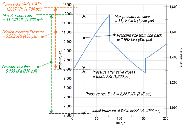
FIGURE 3. To illustrate Example 3, the graph shows the predicted pressure transient at the valve from the system from Figure 2, with pressure rise estimation methods (from Ref. 1)
Now let’s see what happens to the Figure 3 pipeline from a waterhammer point of view when the valve is closed. To determine this, we need additional information as shown here for Example 3, assuming instantaneous valve closure:
a = 1,291 m/s (4,236 ft/s), the wavespeed of the fluid
Δ V = –2.04 m/s (–6.68 ft/s)
Using Equation (3), the Joukowsky pressure rise (ΔPJ) can be determined to be 2,367 kPa (343 psi). This was shown in Equation 7. If an engineer took Equation 3 as the worst-case pressure rise, that person would add this to the initial valve pressure of 6,638 kPa (963 psia) to obtain maximum pressure of 9,005 kPa (1,306 psia). It is true that this would be the pressure rise immediately after the valve closed. However, this is not the maximum pressure, because the pressure will continue to rise after valve closure as the frictional recovery of pressure occurs.
A truly conservative maximum pressure rise can be obtained by adding the two together, as shown in Equation (8):
ΔPmax = ΔPJ + ΔPfr = 5,729 kPa (or 831 psi) (8)
The maximum possible pressure is then obtained by adding the Equation (8) pressure rise to the initial valve pressure (Pvalve). This result is 12,367 kPa (1,794 psia), as shown in Figure 3, where the results from a full transient simulation are also shown. The method in Ref. 7 by Liou is shown also. Here, it is clear that the maximum pressure of 11,967 kPa (1,736 psia) is much higher than what is predicted by Equation (3).
The line pack pressure rise can be seen in Figure 3 from 0 to about 75 s, and totals 2,962 kPa (430 psi). With a keen eye for line pack now at our disposal, look back to the experimental results in Figure 1. After the initial Joukowsky pressure rise of 104 m (340 ft), it is evident that the pressure continues to increase for another 0.1 s or so. This increase is about 5 m (16 ft), which happens to be roughly the frictional pressure loss. Hence, one can see line pack in the Figure 1 experimental results, as well as the simulation results, when one looks closely.
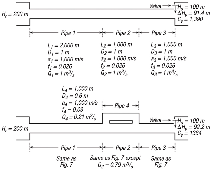
FIGURE 4. The diagrams accompany Example 4, depicting straight (top diagram) and networked (bottom diagram) piping systems (from Ref. 1)
Example 4: Reflected pressure waves. Ref. 1 discusses numerous ways that a reflected wave can cause a pressure rise greater than what would be given by Equation (3). Consider the systems in Figure 4, which shows a straight pipe system and a similar networked system. This example appears in Ref. 1 and was first published in Ref. 8.
In each system in Figure 4, the valve at the end is closed instantly. Figure 5 shows the results. It is clear that the pressure rise in the networked piping is higher than what would be predicted by Equation (1) at 20 s.
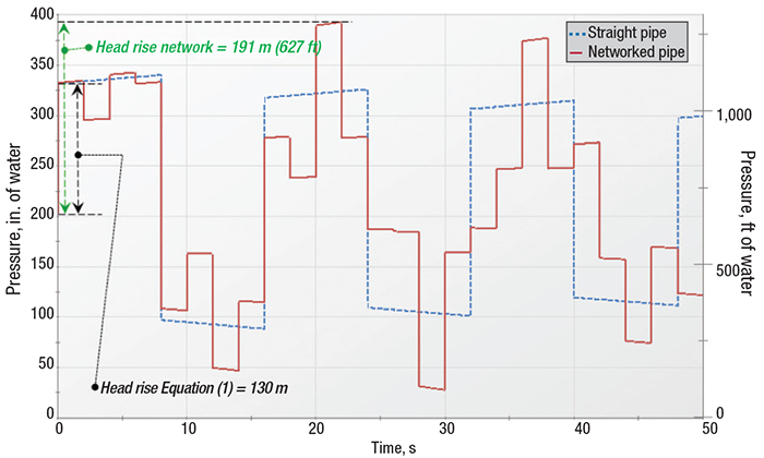
FIGURE 5. Simulation results at the valve from Example 4, using the straight and networked pipe systems in Figure 4 (from Ref. 1)
Numerous other situations can cause reflected waves that exceed the values obtained using Equation (3). These situations include a pipe diameter change, a branch going to a dead-ended pipe and the presence of a gas accumulator [1].
Concluding remarks
Waterhammer can be a complicated issue to address. When possible, a more detailed analysis than the simple Equation (3) should be considered. Ref. 9 provides some guidance to chemical engineers on how to approach this.
The Joukowsky equation is a powerful tool for engineers when used with a proper understanding of its limitations. Engineers should not assume that it always provides a worst-case, conservative pressure rise. The examples presented here clearly show cases where the pressure rise can be much larger than what the Joukowsky equation predicts. Keep this in mind the next time someone tells you they have calculated “the maximum theoretical waterhammer pressure.” Just smile and reply, “are you sure you can trust that?”
Edited by Scott Jenkins
References
1. Walters, T. W. and Leishear, R. A., 2019, “When the Joukowsky Equation Does Not Predict Maximum Water Hammer Pressures,” ASME Journal of Pressure Vessel Technology, Vol. 141 / 060801-1, December 2019.
2. Joukowsky, N., Über den hydraulischen Stoss in Wasserleitungsröhren. (On the hydraulic hammer in water supply pipes), Me´moires de l’Acade´mie Impe´riale des Sciences de St.-Petersbourg, Series 8, Vol. 9, No. 5 (in German, English translation, partly, by Simin, 1904). 1900.
3. Tijsseling, A. S., and Anderson, A., Johannes von Kries and the History of Water Hammer, ASCE Journal of Hydraulic Engineering, Vol. 133, Issue 1, pp. 1–8, 2007.
4. Bergant, A., Simpson, A. R. and Tijsseling, A. S., Water hammer with Column Separation: A Historical Review, Journal of Fluids and Structures, 22, pp. 135–171, 2006.
5. Martin, C. S., “Experimental Investigation of Column Separation With Rapid Closure of Downstream Valve”, 4th International Conference of Pressure Surges, BHRA, pp. 77–88, Bath, UK, 1983.
6. Applied Flow Technology, AFT Impulse 8, Colorado Springs, Colo., USA., 2020.
7. Liou, C. P., Understanding Line Packing in Frictional Water Hammer,” ASME J Fluid Eng, Vol. 138(8), New York, 2016.
8. Karney, B. W., McInnis, D., Transient Analysis of Water Distribution Systems, Journal AWWA, Vol. 82 (7), pp. 62–70, 1990.
9. Prentice, W., 2021, Understand and Mitigate Waterhammer in Fluid Processes, Chem. Eng., March 2021, pp. 28–32.
Author
 Trey Walters is the founder and president of Applied Flow Technology (AFT; 2955 Professional Place, Suite 301, Colorado Springs, CO 80904; Email: [email protected]; Phone: 1-719-686-1000). Walters founded AFT in 1993. He holds a B.S.M.E. (1985) and M.S.M.E. (1986), both from the University of California, Santa Barbara and is a registered professional engineer. Walters is the original developer of AFT Fathom, AFT Arrow and AFT Impulse and has taught hundreds of training classes on AFT’s software products in twelve countries across every populated continent. He worked previously for General Dynamics in cryogenic rocket design and Babcock & Wilcox in steam/water equipment design. Walters is a fellow of the American Society of Mechanical Engineers.