Working with supercritical fluids poses challenges when designing heat exchangers. Some practical tips and precautions are presented here
Industrial applications involving fluids at high pressure — pressure above the critical pressure of a particular fluid — are increasing in number. This is due to the beneficial properties of supercritical fluids (SCFs) or simply due to very high pressures required for certain applications. Examples include supercritical CO2 acting as a solvent in an extraction process, supercritical water for waste treatment via an oxidation process (Figure 1), supercritical nitrogen for an enhanced-oil-recovery process or supercritical methane in compressed natural-gas service. Table 1 provides a list of the critical points for a number of different fluids [1]. The phase diagram for CO2, the most commonly used SCF, is shown in Figure 2.
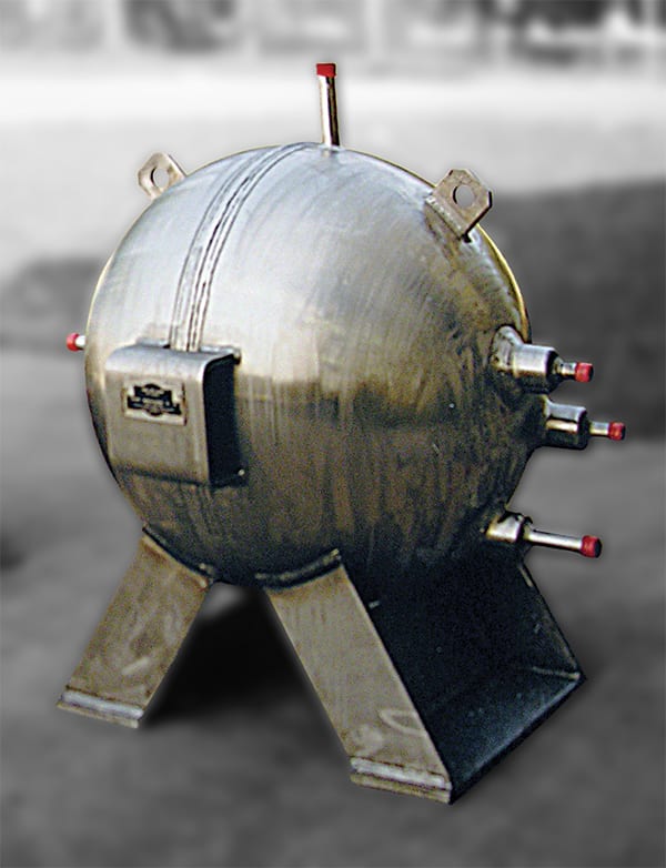
Figure 1. This heat exchanger is used for supercritical water oxidation service. Both hot and cold fluids operate above critical pressure Graham
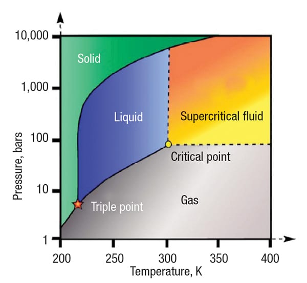
Figure 2. The phase diagram for carbon dioxide illustrates the location of the critical point
Proper design of heat transfer equipment requires greater care and a deeper understanding of supercritical fluid properties, and in particular, how those properties may vary as temperature changes. This article provides design considerations for heat exchangers in supercritical service in order to achieve reliable process performance.
Thermal duty
When presented with supercritical design requirements, an initial step is to determine the thermal duty of the heat-exchanger, Q. Under normal conditions, this is most commonly expressed as Equation (1).
![]() (1)
(1)
Where:
m· = mass flowrate
C p = average specific heat capacity
∆ T = temperature change
It is common for an end user that is requesting a design to provide fluid properties, such as the average heat capacity, at the average temperature. In supercritical service, this can lead to an incorrect determination of thermal duty. Instead, the best practice is to calculate thermal duty considering change in enthalpy, ∆h, as shown in Equation (2).
![]() (2)
(2)
Specific heat can greatly vary with temperature when operating in the supercritical region. For this reason, the change in enthalpy is the most appropriate term for determining the thermal duty. This is best illustrated via an example. Consider a supercritical CO2-extraction application where CO2 at 1,450 psia (1,000 kPa) and a mass flowrate of 11,023 lb/h (5,000 kg/h) must be heated from –10°F to 150°F (–23.3 to 65.6°C). The specific heat capacity of CO2 at the average temperature is 0.637 Btu/lb°F (0.637 kcal/kg°C). The enthalpy at the inlet and outlet temperatures are 63.3 Btu/lb (35.2 kcal/kg) and 189.4 Btu/lb (105.2 kcal/kg), respectively.
Using enthalpy change, [Equation (2)] the thermal duty is 11,023 × (189.4–63.3) = 1,390,000 Btu/h (350,000 kcal/h).
One can see that by using Equation (1) with an average specific-heat capacity and temperature change, the thermal duty is 1,123,500 Btu/h (283,150 kcal/h) or 81% of the true required duty determined by Equation (2). For such a case, a heat exchanger would be undersized by approximately 20% if the thermal duty using average specific heat was applied.
Temperature versus thermal duty
Best practice is to graph temperature change and heat release to understand the shape of the curve. Supercritical fluids can have surprisingly shaped curves caused by property variation as temperature changes. In many services, supercritical fluids will have nonlinear temperature versus thermal-duty curves, such as seen in Figure 3 [2]. This is especially relevant when operating conditions are between the critical pressure and pseudocritical pressure. First we should define these terms.
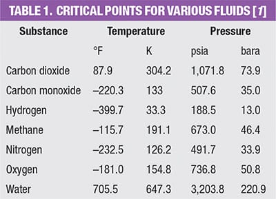
Figure 3. This temperature versus thermal duty graph shows the non-linearity of CO2 curve when heating CO2 at a pressure of 1,450 psia
Critical pressure is the pressure above which a fluid is amorphous; that is, where there is not a distinction between liquid and gas phases, regardless of the temperature. Pseudocritical pressure and temperature is a point where the specific-heat capacity reaches a maximum value. There is great variation in specific heat capacity when, at a given pressure (isobar), the temperature approaches, reaches and surpasses the pseudocritical temperature. Let’s return to Figure 3, which shows a supercritical-CO2 -heating application with water as the heating fluid. The temperature versus thermal-duty curve follows with CO2 heated from –10°F to 150°F, and water cooled from 240°F to 140°F.
Notice that for CO2, the shape of the curve is nonlinear. Common thinking is that the shape of the heating curve is linear, which is true for most sensible-heating applications. The nonlinear shape in supercritical fluid service is due to the large variation in enthalpy and, therefore, specific heat capacity as the CO2 is heated. In this instance, the supercritical CO2-heating curve bends into the water curve, thereby, reducing the effective mean-temperature difference.
Conventional methods for countercurrent flow would determine the log mean-temperature difference (LMTD) using terminal temperature difference with a classic calculation as given by Equation (3)
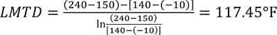 (3)
(3)
Due to the shape of the CO2 curve, a classic LMTD calculation will overstate the effective mean-temperature difference (MTD). In this example, it overstates MTD by 13%, as the next calculation shows.
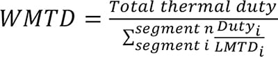
Best practice is to apply a segmental approach, breaking the temperature curve into segments of smaller temperature changes and applying LMTD calculation for each step. This yields a duty-weighted, mean-temperature difference (WMTD), shown in Equation (4).
 (4)
(4)
Using 10 segments, one for each 16 degree rise in CO2 temperature, Equation (4) yields WMTD = 103.7°F.
For reliable performance and accurate heat-exchanger sizing, always consider using the WMTD calculation when the temperature profile is nonlinear.
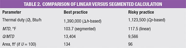
Consider together thermal duty and LMTD and how dramatically different the heat-exchanger selection will be. When average specific heat is used, coupled with a classic LMTD, and that is compared to an enthalpy based thermal duty with a segmental WMTD, that concern for great care is apparent. Assuming the overall heat-transfer coefficient (U) is the same in either case, the required surface area differs by 40% (see Table 2).
Two additional examples comparing WMTD and LMTD are shown in Figure 4, which reinforces the risk associated with using the linear LMTD calculation and how the WMTD calculation yields a different number. The key take-away here is to plot the duty versus temperature and perform a segmented WMTD calculation to get it correct.
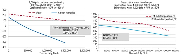
Figure 4. Shown here are two examples of non-linear behavior of temperature versus thermal duty, and the resulting values calculated for WMTD and LMTD
It is also interesting to compare the shape of the CO2 heating curve for the very same temperature change from –10 to 150°F for three different isobars, as shown in Figure 5. A pressure of 725 psia is below the critical pressure. As the CO2 is heated, there is sensible heating of liquid CO2 up to the boiling temperature of 57.7°F. This is followed by isothermal boiling until all of the CO2 is vaporized, and then gas sensible superheating to 150°F. In contrast, at a pressure of 3,000 psia, which is well above the critical pressure, the heating curve is close to linear and comparable to a sensible heating. For the 1,450-psia case, which is near to critical pressure, the shape of the heating curve is nonlinear and atypical.
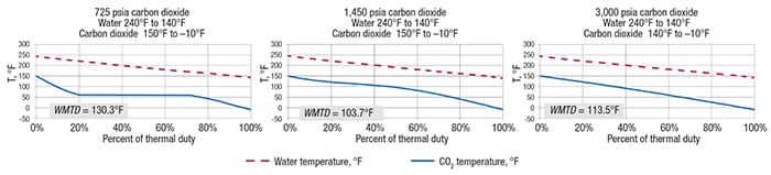
Figure 5. Shown here are the heating curves for CO2 at three different pressures
Fluid property variation
There can be wide variation in fluid properties, such as density, specific heat capacity, viscosity and thermal conductivity, between the inlet and the outlet temperature. Again, when operating between the critical pressure and the pseudocritical pressure, the specific heat may vary greatly with temperature. Good practice is to graph the fluid properties as a function of temperature to understand how extreme the variation might be. At a pressure well above the critical pressure and beyond the pseudocritical pressure, such a wide variation is reduced. Referring again to the 1,450 psia supercritical CO2 example (Figure 5), the graph shown in Figure 6 depicts how fluid properties vary from an inlet temperature of –10°F to an outlet temperature of 150°F. Specific heat capacity stands out. Noteworthy is the pseudocritical point, which is 1,450 psia and approximately 110°F. Specific heat reaches a maximum at the pseudocritical point and is lower on either side of this point. The graph provides comparison for how properties vary up or down from properties determined at average temperature of 70°F (the average of –10°F and 150°F).
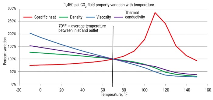
Figure 6. Near the pseudocritical pressure, physical properties vary considerably as a function of temperature, especially the specific heat
Heat transfer coefficient
Supercritical fluids are often on the tubeside of a heat exchanger due to the high operating pressure, which is mechanically easier to contend with on the tubeside. Fluid properties directly influence the heat-transfer coefficient. When applying a classic Nusselt equation for in-tube flow at turbulent conditions, one can identify how a local heat-transfer coefficient is impacted by fluid properties, by the relationship between the Nusselt number, Nu, Reynold number, Re, and Prandtl number, Pr:
![]() (5)
(5)
Expression (5) reduces to Expression (6), which shows the relation between the tubeside heat-transfer coefficient, HTC, and the physical properties of viscosity, η, thermal conductivity, κ and specific heat, CP:
![]() (6)
(6)
From the graph shown in Figure 6, the specific heat variation greatly affects HTC, as does the viscosity and the thermal conductivity.
Research with supercritical fluids has found there can be significant radial property variation within a tube between average bulk temperature properties and those at the tube-wall temperature. There are factors one might apply to reflect the impact of bulk and tube-wall fluid properties for density, specific heat and viscosity.
Further to a segmental approach used to determine WMTD, it is recommended that HTC is considered segmentally as well to capture HTC variation along the temperature change. The graph shown in Figure 7 illustrates that, for 1,450 psig CO2, the calculated HTC variance is 87% at the inlet, 157% near the pseudocritical point and 90% at the outlet compared to the HTC determined at the average temperature of 70°F. This observation supports using a segmental approach (or discretization of temperature change) to capture correctly the local LMTD and HTC.

Figure 7. The variation of Re, Pr and HTC as a function of temperature is shown here for CO2 at 1,450°C
As noted previously, the bulk or average fluid properties can vary significantly from the fluid properties at the tube wall. Such variation will also influence HTC. The following equations are used for determining tubewall temperature on the inside (supercritical fluid side) and outside surface.
![]() (7)
(7)
![]() (8)
(8)
Where:
Twall,ID = Tubewall temperature at the inside surface of the tube
Twall,OD = Tubewall temperature at the outside surface of the tube
TTS = Tubeside bulk temperature
TSS = Shellside bulk temperature
U = Overall heat transfer coefficient
HTC = Supercritical fluid heat-transfercoefficient
HSS = Shellside heat transfer coefficient
Let’s return to the CO2 heating application at 1,450 psig. By applying a segmental analysis with 10°F increments, we can compare the bulk or average temperature to the temperature of the tubewall inside diameter. There can be order-of-magnitude differences between bulk and tubewall properties when working with supercritical fluids. The graph shown in Figure 8 plots the tubewall temperature along the heat curve and illustrates how the fluid properties vary greatly between the bulk and those at wall temperature.
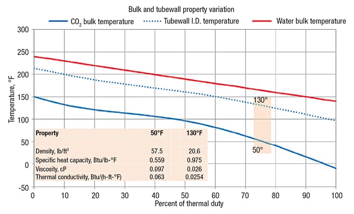
Figure 8: This graph shows the variation of properties in the bulk and at the tubewall as a function of temperature
Some literature suggests using film-temperature properties. Film temperature is commonly considered to be the average of segment bulk and tubewall temperatures. Other literature applies correction factors for variation in specific heat and density. The author suggests applying physical properties that directionally drive the calculated HTC lower to provide a degree of safety. Film temperature serves as a good surrogate for determining what properties to apply. The author further suggests comparing bulk and film properties and using that property that yields a lower calculated HTC. If, however, the design provides adequate safety factors, such as, for example, a 60% cleanliness factor or a 50% excess area, then using film temperature for fluid properties is adequate.
Each supercritical fluid is unique, and the temperature-pressure region where a nonlinear thermal-duty curve is most likely will depend on a given fluids’ properties. The closer the operating pressure is to the critical pressure, the more variation in specific heat as temperature changes is to be expected. Carbon dioxide has a critical pressure of 1,072 psia. Figure 9 illustrates how specific heat varies as temperature varies for different isobars. Note that the specific heat of 1,100 psia CO2, which is just slightly greater than the critical pressure, is 29.72 Btu/lb°F when the temperature is 90°F. Recall a previous definition for pseudocritical temperature and pseudocritical pressure that describes where specific heat is a maximum. This is shown as the apex for each isobar in the graphs shown in Figure 9.
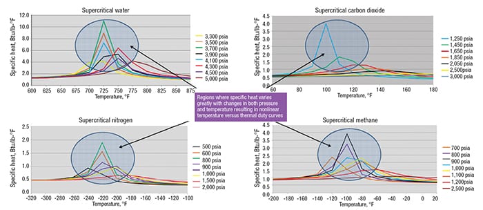
Figure 9. These graphs show the variation of specific heat with temperature at several isobars for four different fluids. The shift of the pseudocritical temperature can be observed
Summary
Supercritical fluid heat transfer warrants more careful consideration than normally needed for more traditional heat-exchanger designs. This is due to fluid property variations when operating above the critical point and for a given isobar when the operating temperature is near to, or passes through the pseudocritical temperature. At a pressure well above the critical point there is less concern as property variation is not as significant. Key design considerations include the following:
- Determine the thermal duty of a supercritical fluid using enthalpy change
- Graph temperature versus thermal duty to understand shape of the curve
- When warranted, perform a segmental analysis to capture correctly WMTD and within each segment to determine surface area necessary based on segment thermal duty, segment LMTD and segment HTC
- Evaluate bulk and wall property variation to determine if further HTC refinement is necessary
References
1. Van Wylen, Gordon J. and Sonntag, Richard E., “Fundamentals of Classical Thermodynamics,” Wiley, Hoboken, N.J., 1993.
2. All fluid-property modeling used to generate the graphs was done using NIST REFPROP webbook, https://webbook.nist.gov/chemistry/name-ser.
Author
 James R. Lines is president and CEO of Graham Corp. (20 Florence Ave., Batavia, N.Y. 14020; Phone: 585-343-2216; Fax: 585-343-1097; Email: jlines@graham-mfg.com), a position he has held since 2008. Prior to that, Lines served as president and COO and as a director of the company. He has been working at the company in various capacities since 1984, holding positions of vice president and general manager, vice president of Engineering, and vice president of Sales and Marketing. Prior to joining the management team, he served as an application engineer and sales engineer as well as a product supervisor. Lines holds a B.S. in aerospace engineering from the State University of New York at Buffalo. The author’s company has designed and successfully supplied its Heliflow heat exchangers in supercritical service for carbon monoxide, carbon dioxide, nitrogen, hydrogen, oxygen, methane, water and various other fluids.