In order to correctly size pressure relief valves (PRVs), a robust understanding of discharge coefficients for vapor, liquid and two-phase flow is crucial
A pressure relief valve (PRV) is used to prevent the pressure in a process vessel from exceeding the allowed pressure rating of the vessel. The required PRV orifice area is determined by dividing an ideal nozzle orifice area by a valve discharge coefficient. Therefore, proper use of PRV discharge coefficients is very important for sizing PRVs and preventing potential overpressure of process vessels.
PRV manufacturers provide certified discharge coefficients that were determined experimentally for liquids and vapors. Certified PRV discharge coefficient values are reported in the Pressure Relief Device Certifications, NB-18 [ 1] from the National Board of Boiler and Pressure Vessel Inspectors. The certifications are based on isentropic ideal nozzle-flow equations for incompressible flow of water and compressible flow of air and steam. However, there is no certified discharge coefficient for two-phase flow. As many others have noted in the literature, the authors have found that the discharge coefficient for gases is significantly greater than the discharge coefficient for liquids.
The authors have revisited a previous theory on PRV discharge coefficients and investigated manufacturers’ information and experimental data readily available in the literature. This article presents a new theory for explaining the significant difference between liquid and vapor discharge coefficients. This article also provides guidelines for the proper use of PRV liquid and vapor discharge coefficients for liquid, vapor and two-phase flow.
PRV nozzle discharge coefficient
A theoretical flow model assumes frictionless isentropic flow. In reality, the actual measured flow capacities of PRVs deviate from the calculated theoretical ideal nozzle-flow capacities. The discharge coefficient accounts for the difference between the mass flux in the actual valve and that calculated by the theoretical flow model. The coefficient of discharge is given in Equation (1), which defines the discharge coefficient (Kd) of a PRV as the ratio of the measured flow capacity through the valve (GM) to its theoretical ideal nozzle-flow capacity (GT).
Kd = GM / GT (1)
Thus, the discharge coefficient is dimensionless and normally less than 1. The PRV sizing standard API 520 recommends the typical value of 0.975 for sizing PRVs for vapor service. On the other hand, the typical value of 0.65 is recommended for sizing PRVs for liquid service. For sizing PRVs for two-phase service, there is no typical value recommended by API 520 or by valve manufacturers.
National Board PRV certifications
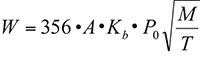
NB-18 (Relief Device Certifications) provides a complete listing of and information pertaining to pressure-relief device designs that are certified by the National Board. The capacity of a PRV is certified by one of two ASME methods — the slope method or the coefficient method. The authors have reviewed the ASME Section VIII Div.1 PRV certified values that were determined by the coefficient method. The publication includes the discharge coefficients for vapor and liquid flows. The ASME theoretical flow capacity for water (incompressible fluid) and air (compressible fluid) are defined by Equations (2) and (3), respectively. This article only considers two equations for water and air. Das [ 2] presented all the details of the ASME discharge coefficients in his article. The measured coefficient of discharge defined by Equation (1) is multiplied by 0.9 (derating factor) to obtain the ASME-certified discharge of coefficient K defined by Equation (4).
W = 2,407 · A · [( P – P d) · w] 0.5 (2)
W = 356 · A · P · (M/ T) 0.5 (3)
K = 0.9· Kd (4)
Where:
W = theoretical flow capacity, lb/h
A = nozzle throat area, in.2
P = Set pressure × 1.1 + atmospheric pressure, or set pressure + 3 psi + atmospheric pressure (whichever is greater), psia
Pd = pressure at discharge from device, psia
w = water density at device inlet conditions, lb/ft3
M = molecular weight
T = absolute temperature at device inlet conditions, R
Kd = actual (or measured) coefficient of discharge
K= ASME certified coefficient of discharge (derated)
Figure 1 shows all K values of PRVs that were certified as per ASME Section VIII. As can be seen, the distribution of the K values for liquid (water) is widely spread. On the other hand, there is a relatively high distribution of K values for vapor (air) that are greater than 0.85. It is apparent that certified vapor discharge coefficients (average: 0.833) are greater than liquid discharge coefficients (average: 0.671). If a valve is certified for both liquid and vapor, the liquid K is generally smaller than the vapor K.
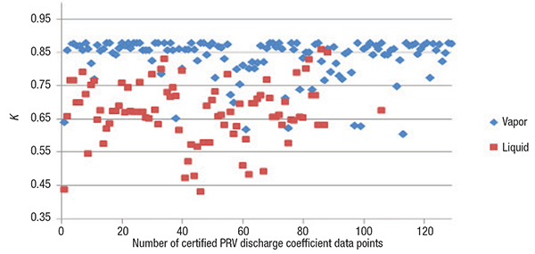
Figure 1. PRV discharge coefficient values (K) are certified according to ASME Section VIII for
vapor and liquid
Figure 2 shows all vapor K values of conventional and pilot-operated PRVs that were certified as per ASME Section VIII. The major difference between conventional and pilot-operated relief valves is that conventional relief valves use a spring to close the valve and pilot-operated valves use the inlet gas pressure to keep the valve closed. Therefore, the top area of the piston for pilot-operated valves is designed to be larger than the inlet, and there is a constant force difference keeping the valve closed. As seen in Figure 2, the lowest certified discharge coefficient is 0.604. A few vapor K values are not greater than the average certified liquid K value. Both types have a highest value of 0.878. The certified vapor discharge coefficients (average: 0.839) for pilot-operated PRVs are slightly greater than the vapor discharge coefficients (average: 0.830) for conventional devices.
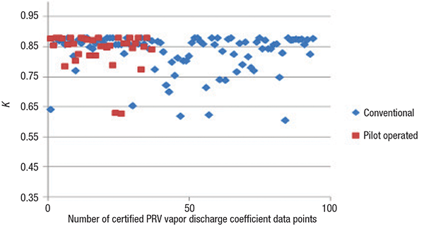
Figure 2. Due to their differing closing mechanisms, conventional and pilot-operated PRVs
exhibit slightly different K values
Figure 3 shows all liquid K values of conventional and pilot-operated PRVs that were certified as per ASME Section VIII. The lowest liquid discharge coefficient is 0.431. The highest liquid discharge coefficient is 0.857. A few liquid K values are greater than the average vapor certified K. The certified liquid discharge coefficients (average: 0.733) for pilot-operated PRVs are greater than the certified liquid discharge coefficients (average: 0.644) for conventional PRVs.
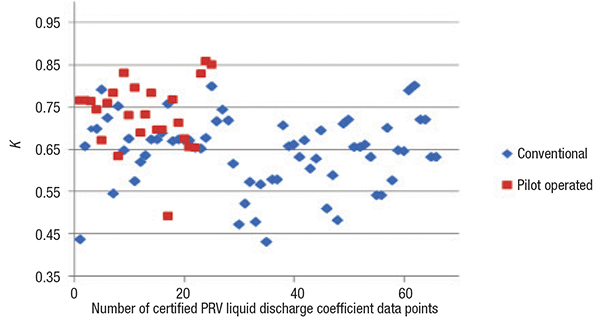
Figure 3. For liquids, the certified K values of pilot-operated PRvs are generally larger than those for conventional-type PRVs
Review of existing knowledge
For single-phase flow, the certified values of discharge coefficients are available from valve manufacturers and are used for sizing PRVs. Darby [3] states that the vapor discharge coefficient is significantly greater than the liquid discharge coefficient, because vapor flow is measured under choked conditions. Since vapor flow under subcritical conditions and liquid flow do not choke, the entire valve affects the mass flux, resulting in a lower discharge coefficient value.
For two-phase flow, the certified values of discharge coefficients are not available from valve manufacturers. Two-phase discharge coefficients were reviewed by Lenzing [ 4], Leung [ 5] and Darby [ 6]. Equation (5) is generally used for the estimation of the two-phase discharge coefficient. However, there is no appropriate flow model that can accurately predict two-phase flow in PRVs. Darby suggested that the vapor discharge coefficient be used for choked two-phase flow and the liquid discharge coefficient be used for non-choked two-phase flow.
Kd TP = a· KdG + (1 – a)· KdL (5)
Where:
KdTP = Two-phase discharge coefficient
a = Vapor volume fraction
KdG = Vapor-phase discharge coefficient
KdL = Liquid-phase discharge coefficient
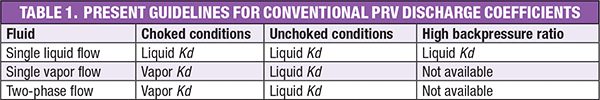
The present guidelines on the proper use of discharge coefficients for PRVs can be summarized as shown in Table 1.
Why KdG is greater than KdL
Comflow (Compressible Flow) and TPHEM (Two-phase Homogeneous Equilibrium Model) are computer programs used to estimate flowrate and pressure changes in ideal nozzles and piping systems. These programs are available with the Center for Chemical Process Safety (CCPS) guideline book [ 7]. The help files on these programs recommend that the pipe exit loss for vapor (compressible) and two-phase flows should not be considered. This is because there is generally no pipe exit loss for compressible fluid. On the other hand, exit loss should be considered for liquid (incompressible) flow.
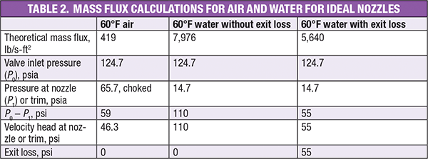
Figure 4 presents PRV details showing the area of the smallest nozzle cross-section ( AN, nozzle flow area) and the area of the trim cross-section ( AT, trim annular flow area) determined by lift. Table 2 is a summary of mass flux calculations for air and water for ideal nozzles. All calculations assume that there is no friction in the valve. The pressure drop from the nozzle throat to the valve trim affects the valve discharge coefficient. It is also assumed that both the effective nozzle area and trim area are identical. So if there is an exit loss for water (incompressible fluid), the available differential pressure for mass flux will be 50% of the total available differential pressure.
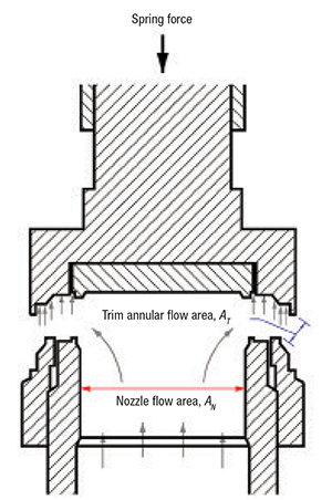
Figure 4. PRV nozzle flow area and trim flow area are important parameters to consider for mass flux calculations
For air (compressible fluid), the velocity head (46.3 psi) at the nozzle or trim is much smaller than the available differential pressure (59 psi). Generally, all available differential pressure is supposed to be converted to the velocity head at the nozzle. However, there is a significant gap (12.7 psi) between the values, because of significant changes in compressible fluid density during an expansion process. The authors consider no exit loss for compressible flow, because this pressure gap is able to move fluid forward without exit loss. On the other hand, the velocity head for incompressible flow is equal to the total available differential pressure. This means that the incompressible fluid needs some extra pressure to exit the valve. This extra pressure is the valve exit loss for incompressible fluids. As can be seen in Table 2, the exit loss for incompressible flow significantly influences the mass flux, resulting in a liquid discharge coefficient (5,640/7,976 = 0.707) that is lower than the vapor discharge coefficient.
KdG for subcritical flow
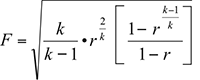
The authors have revisited the calculation methods for gases under subcritical conditions to check the actual coefficient of discharge for superheated air at 124.7 psia and 60°F. The theoretical mass flux for subcritical vapor flow can be determined using either Equation (6) or (8) below.
![]() (6)
(6)
 (7)
(7)
 (8)
(8)
Where:
W = valve flow capacity for air, lb/h
A = nozzle throat area, in.2
F = coefficient of subcritical flow
M = 29, molecular weight, g/mol
T = 520, absolute temperature at device inlet conditions, R
P 0 = upstream relieving pressure, psia
P 2 = backpressure, psia
k = 1.4, ratio of the specific heats for an ideal gas at relieving temperature
r = ratio of backpressure to upstream relieving pressure
K b = backpressure correction factor
Equation (8) is necessary to account for the backpressure effect on the mass flux. The backpressure correction factor is normally provided by valve manufacturers. The mass flux at subcritical conditions is less than the choked mass flux because the compressible fluids reach a maximum flow at choked conditions.
Table 3 shows the mass flux results determined by Equations (6) and (8). Both calculations assume a valve discharge coefficient of 0.95 and a backpressure of 94.7 psia. As can be seen, the two calculation results for subcritical flow are in good agreement. This indicates that there is negligible pressure drop downstream of the valve nozzle. If the backpressure correction factor is smaller than 1 at a lower backpressure ratio than the choked conditions (r = 0.53), then there is pressure drop downstream of the valve nozzle. Therefore, the API 520 [ 8] backpressure correction factor is based on a negligible pressure drop downstream of the valve nozzle.
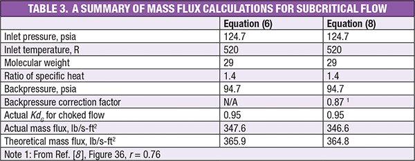
Figure 5 plots the values of the calculated discharge coefficient for two conventional PRV models: Consolidated 1900 (Valve 1; KdG = 0.95; KdL = 0.744); and Pentair JLT-JOS (Valve 2; KdG = 0.967; KdL = 0.729) based on their backpressure correction factors [ 9, 10]. Leung [ 5] has presented that KdG coincides with KdL at an absolute backpressure ratio of 1.0. As can be seen, the calculated discharge coefficients of Valve 1 are constant, except at the backpressure ratio of 0.95. The vapor KdG is generally constant and independent of the backpressure ratio. This means that the valve is designed with negligible pressure drop downstream of the valve nozzle. The vapor discharge coefficient for subcritical conditions and high backpressure ratios is determined by the corresponding pressure drop ( P1 – P2) downstream of the valve nozzle and the actual mass flux per unit pressure driving force ( MPUP), defined as the actual mass flux divided by the difference between P0 and P1. The MPUP variation is inherent for compressible flow. The final Valve 1 Kd value (at the backpressure ratio of 0.95) decreases slightly because it has the highest MPUP, as shown in Table 4. Although Valve 1 is designed with negligible pressure drop, the high MPUP results in a small pressure drop downstream of the valve nozzle, which leads to a slightly lower Kd value. For Valve 2, the Kd value varies with the backpressure ratio. As shown in Table 5, Valve 2 is designed with significant pressure drop downstream of the valve nozzle, so the discharge coefficient for subcritical conditions decreases as the backpressure ratio increases. However, the vapor Kd at the backpressure ratio of 0.95 is smaller than the liquid discharge coefficient. Therefore, there is probably no link between KdG and KdL. Compressible fluids are essentially different from incompressible fluids.
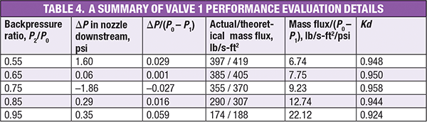
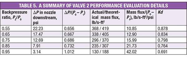
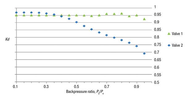
Figure 5. This plot of KdG variation with backpressure ratio for conventional PRVs shows how different valve models are impacted by backpressure ratio
For incompressible flow, the MPUP is constant regardless of the backpressure ratio, so the liquid Kd value remains constant. Interestingly, the liquid Kd value of 0.744 is much smaller than the vapor Kd value. Thus, the liquid Kd value of 0.744 only can be explained by the valve exit loss required for incompressible (liquid) flow. If there is significant pressure drop downstream of the valve nozzle without an exit loss, the PRV will not function properly. The significant pressure drop may close the valve. However, the exit loss does not affect the function of valve opening and closing.
Tables 4 and 5 summarize the calculation details for Valve 1 and Valve 2 under subcritical conditions. All the calculations are based on the assumption that the certified actual Kdvalue is valid up to the valve nozzle throat.
Review of experimental data
Lenzing and others [ 4] presented both air-water and steam-water experimental data for the ASME-certified PRV model Leser DN25/40 441. The authors have reviewed the experimental data to evaluate the discharge coefficients for single flow, non-flashing two-phase flow and flashing two-phase flow using Equations (9) through (11), which are shown below.
Homogenous Equilibrium Equations
 (9)
(9)
![]() (10)
(10)
 (11)
(11)
Where:
P ec = Pressure at equivalent choked (critical) conditions, psia
G = Mass flux, lb/s-ft 2
v = Specific volume, ft 3 /lb
∝, β = Parameters for a pressure-specific volume correlation
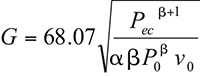
Equation (9) was used to estimate the theoretical mass flux ( G) for all flows in terms of Pec, the pressure at equivalent choked (critical) conditions, which is defined by Equation (10). The theoretical mass flux was obtained by integrating Equation (11) for homogeneous equilibrium flow based on three data sets of specific volume versus pressure relationships from the stagnation pressure P0 at the vessel to the valve nozzle pressure Pat the throat. Kim and others [ 11] developed the flow model based on homogeneous equilibrium. The authors consider the homogeneous equilibrium model (HEM) to be the most appropriate and conservative model for relief valve sizing currently available.
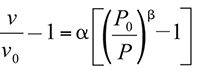
Using a pressure-specific volume relationship, such as Equation (11), in nozzle flow calculations can greatly simplify the complexity of the flow calculations. Equation (11) requires three specific-volume data points at P0 (vessel pressure) and P1 (middle pressure, ( P0 + P2)/2) and P 2 (atmospheric pressure) to solve for the parameters α and β. Equation (11) gives outstanding fits of the data for gases and two-phase systems. The specific volume data sets are generally obtained by isentropic flash calculations. Equation (11) is used to predict specific volumes during the isentropic expansion process in PRVs.
Figure 6 shows the measured discharge coefficients for the Leser DN25/40 441 valve for air-water flow at 72.495 psia (5 bars). The air-water data covers a limited set of data points in the range of 0.0001 ≤ x o ≤ 1, where x o is the inlet air quality in weight fraction. The theoretical mass fluxes are based on isentropic flow in thermal equilibrium. The certified actual discharge coefficients of vapor and liquid are 0.777 and 0.579, respectively. The flow behaves as if it were incompressible when the air quality is 0.0001. The flow behaves as if it were compressible when the air quality is greater than 0.001. The incompressible-compressible transition occurs at 0.0001 < x o < 0.001. Although the measured values are generally greater than the certified discharge coefficients, all data points except two (at x o = 0.00236 and x o = 0.0045) are in relatively good agreement with the certified actual discharge coefficients. These two data points may suggest some experimental problem.
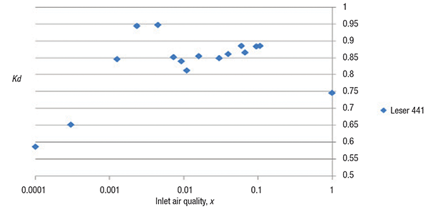
Figure 6. Measured Kd values of the Leser 441 PRV for air-water data at 72.495 psia are shown
Figure 7 shows the measured discharge coefficients for the Leser DN25/40 441 valve for 153.74 psia (10.6 bars) steam-water flow. The steam-water data covered a limited set of data points in the range of 0.0011 ≤ x o ≤ 1. The theoretical mass fluxes are based on the isentropic flow in thermal equilibrium. The certified actual discharge coefficients of vapor and liquid are 0.777 and 0.579, respectively. All the flashing two-phase data points lie significantly outside of the upper tolerance of the vapor discharge coefficient. Thermal non-equilibrium effects would be the main cause of a higher measured Kd value than the certified actual vapor Kd. The non-equilibrium effect diminishes with increasing inlet vapor mass fraction. The equilibrium flow model under-predicts mass flux over all of the flashing two-phase data points.
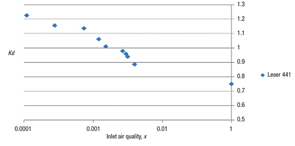
Figure 7. Measured Kd values of the Leser 441 PRV for steam-water data at 153.74 psia are shown
To help clarify the calculation process and concepts, three example calculations for liquid flow, vapor flow and two-phase non-flashing flow are shown below. The example data were selected from an experimental data set of Lenzing and others [ 4].
Example calculations
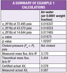
Example 1
Example 1 considers an air-water system (inlet air mass fraction = 0.0001) at 72.495 psia (5 bar) and 77°F. The stagnation pressure of the fluid entering the Leser type 441 valve nozzle is 72.495 psia. The stagnation temperature is 77°F. The backpressure on the relief valve is 14.644 psia. All physical properties used and the results calculated with the universal mass flux equation are listed in the summary table.
Step 1. Calculate the Pec using Equation (10) at the system backpressure of 14.644 psia and the data given in Table 6. This yields a Pec of 11.53 psia. The flow is unchoked because the calculated Pec is not greater than 14.644 psia.
Step 2. Calculate the mass flux at the Pec of 11.53 psia using Equation (9). This gives a value of 5,404 lb/s-ft 2.
Step 3. Calculate the valve coefficient of discharge using Equation (1). Dividing the measured flux (3,170) by the theoretical flux from the previous step (5,404) results in a Kd of 0.587. This flow appears to be incompressible flow based on the measured Kd value.
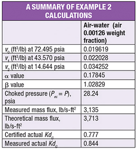
Example 2
Example 2 considers an air-water system (inlet air mass fraction = 0.00126) at 72.495 (5 bar) and 77°F. The stagnation pressure of the fluid entering the Leser type 441 valve nozzle is 72.495 psia. The stagnation temperature is 77°F. The backpressure on the relief valve is 14.644 psia. All physical properties used and the results calculated with the universal mass flux equation are listed in the summary table.
Step 1. Calculate the Pec using Equation (10) and the data from Table 7 at the system backpressure of 14.644 psia. This results in a Pec of 24.86 psia. The flow is choked because the calculated P ec is greater than 14.644 psia.
Step 2. Repeat Step 1 to seek the choked pressure by substituting the previous approximation ( Pec) as P into Equation (10) until the Pec is approximately P. In this example, the fourth trial resulted in a Pec of 28.24 psia.
Step 3. Calculate mass flux at the choked pressure of 28.24 psia using Equation (9). For this example, the mass flux is 3,713 lb/s-ft 2.
Step 4. Calculate the valve coefficient of discharge using Equation (1), which gives a Kd of 0.844. This flow appears to be compressible flow based on the measured Kd value.
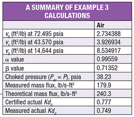
Example 3
Example 3 considers air at 72.495 psia (5 bar) and 77°F. The stagnation pressure of air entering the Leser type 441 valve nozzle is 72.495 psia. The stagnation temperature is 77°F. The backpressure on the relief valve is 14.644 psia. All physical properties used and the results calculated with the universal mass flux equation are listed in the summary table.
Step 1. Calculate the Pec using Equation (10) at the system backpressure of 14.644 psia. The calculated Pec is 27.23 psia. The flow is choked because the calculated Pec is greater than 14.644 psia.
Step 2. Repeat step 1 to seek the choked pressure by substituting the previous approximation ( Pec) as P into Equation (10) until the Pec is approximately P. The fifth trial gave a Pec of 38.23 psia.
Step 3. Calculate mass flux at the choked pressure of 38.23 psia using Equation (9). The calculated mass flux is 240.3 lb/s-ft 2.
Step 4. Calculate the valve coefficient of discharge using Equation (1). Here, the calculated Kd is 0.749, indicating that the flow is compressible.
Final recommendations
Based on the data and calculations presented in this article, the authors recommend the following as a guide to proper use of conventional PRV discharge coefficients. These guidelines are also summarized in Table 6.
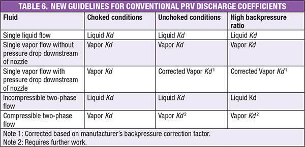
Single liquid flow.Size a PRV based on the ASME-certified liquid discharge coefficient that was determined experimentally. The liquid K is constant regardless of the backpressure ratio.
Single vapor flow. Size a PRV based on the ASME-certified vapor discharge coefficient that was determined experimentally for choked flow. The vapor K can vary significantly with the backpressure ratio if the valve is designed with pressure drop downstream of the valve nozzle. Therefore, the backpressure correction factor provided by the valve manufacturer should be used to size the PRV if the backpressure correction factor is less than 1.0 at lower backpressure ratio than choked conditions.
The vapor discharge coefficient for subcritical conditions and high backpressure ratios is determined by the actual MPUP and the corresponding pressure drop downstream of the valve nozzle. The changes in Kd are due to a variation in the MPUP. The MPUP variation is inherent for compressible flow. For incompressible flow, the MPUP is constant regardless of the backpressure ratio, so the liquid Kd value remains constant.
On the other hand, the vapor K for choked conditions can be used to size the PRV if the backpressure correction factor is not less than 1.0 at lower backpressure ratio than choked conditions. The vapor Kfor the valves designed with negligible pressure drop in the downstream of the valve nozzle is generally independent of the backpressure ratio.
Two-phase flow.Unlike single liquid and vapor flows, valve manufactures do not provide any discharge coefficient value for two-phase flow. However, PRV sizing should be based on the ASME-certified discharge coefficient for vapor if the fluid behavior is compressible flow. If the fluid behavior is incompressible flow, the ASME-certified discharge coefficient for liquids is recommended to size PRVs. However, many empirical two-phase discharge coefficients are much greater than the vapor Kd. Thermal non-equilibrium is known to be the main cause of such high values. But there is also no accurate flow model that accounts for non-equilibrium. Although this article does not present the non-equilibrium flow model, the authors are developing the non-equilibrium correction factor and the discharge coefficient for transitional flow between compressible flow and incompressible flow. The discharge coefficient of transitional flow may lie between the liquid Kd and vapor Kd.
Finally, the authors propose an exit loss theory to explain why the liquid discharge coefficient is normally smaller than the discharge coefficient of vapor. The exit loss yields a lower liquid discharge coefficient, however, there is no exit loss for vapor flow and two-phase flow with a significant change in density. No exit loss can result in a high certified vapor discharge coefficient maximum of 0.878. ■
Edited by Mary Page Bailey
References
1. National Board Pressure Relief Device Certifications, NB-18, The National Board of Boiler and Pressure Vessel Inspectors, Feb. 2016.
2. Das, D., Discharge Coefficients and Flow Resistance Factors, Chem. Eng., October 2008, pp. 52–59.
3. Darby, R., Meiller, P. and Stockton, J., Select the Best Model for Two-Phase Relief Sizing, Chem. Eng. Prog., May 2001, pp. 56–64.
4. Lenzing, T., Friedel, L., Cremers, J., and Alhusein, M., Prediction of the Maximum Full Lift Safety Valve Two-phase Flow Capacity, Journal of Loss Prevention in the Process Industries, 11, pp. 307–321.
5. Leung, J. C., A Theory on the Discharge Coefficient for Safety Relief Valve, Journal of Loss Prevention in the Process Industries, 17, pp. 301–313, 2004.
6. Darby, R., On Two-Phase Frozen and Flashing Flows in Safety Relief Valves, Journal of Loss Prevention in the Process Industries, 17, pp. 255–259, 2004.
7. Guidelines for Pressure Relief and Effluent Handling Systems, Center for Chemical Process Safety (CCPS), AIChE, New York, 1998.
8. Sizing, Selection, and Installation of Pressure-relieving Devices in Refineries, API Standard 520, Part I – Sizing and Selection, Ninth Ed., Dec. 2013.
9. Pentair Pressure Relief Valve Engineering Handbook, Pentair Technical Publication No. TP-V300, pp. 7.15–7.16.
10. General Information Safety Relief Valve, Consolidated Catalogue, pp. VS.9.
11. Kim, J. S., Dunsheath, H. J. and Singh, N. R., Sizing Calculations for Pressure-Relief Valves, Chem. Eng., Feb. 2013, pp. 35–39.
Authors
 Jung Seob Kim is a principal process engineer at Sunlake Co. Ltd. (Suite 204 5 Richard Way SW, Calgary, Alb., Canada T3E 7M8; Phone: 713-870-8746; Email: jukim@suncor.com) where he is currently supporting the Suncor Energy process engineering team at Fort Hills. He has more than 30 years of experience in different roles within the petrochemicals processing industry, including with SK E&C USA, Bayer Technology Services, Samsung BP Chemicals and Samsung Engineering. He holds a B.S.Ch.E. degree from the University of Seoul, is a member of AIChE and is a registered professional engineer in the state of Texas.
 Heather Jean Dunsheath is a senior process safety engineer at Covestro (8500 West Bay Road MS 21, Baytown, TX 77523; Phone: 281-383-6879; Email: heather.dunsheath@covestro.com). She has more than ten years of experience in process safety, including designing emergency relief systems and facilitating process hazard analysis (PHA) studies. Dunsheath has also co-authored several scientific papers and articles. She holds a B.S.Ch.E. degree from Rice University in Houston.
 Hyun Ji Woo is a process engineer at SK E&C (SK G.plant, 100 Euljiro, Jung-gu, Seoul, 100-847, Korea; Phone: 82-2-3499-2967; Email: hj.woo@sk.com) where she has about nine years of experience in designing refinery plants. She holds a B.S.Ch.E. degree from Hanyang University in Seoul, Korea.
 Nayeon Kim is a Process engineer at SK E&C (SK G.plant, 100 Euljiro, Jung-gu, Seoul, 100-847, Korea; Phone: 82-2-3499-2072; Email: iloveny@sk.com) where she has about six years of experience in designing refinery plants. She holds a B.S.Ch.E. degree from Sungkyunkwan University in Seoul, Korea.